RecSys Auto Research KB
A knowledge base for recommender-system auto research · from cascading architectures to the generative paradigm





A knowledge base for recommender systems and computational advertising: discriminative recommendation, generative recommendation, and the advertising stack — structured, citable technical knowledge for auto research by humans and AI agents.
What Is This?
RecSys Auto Research KB is a knowledge base for recommender-system auto research, rewritten and expanded from the Datawhale open-source project fun-rec.
📖 Read online: visit https://haozhe-xing.github.io/fun-rec-mdbook/ for the latest version.
The book follows two main threads:
- Discriminative recommendation: retrieval, ranking, re-ranking, multi-task learning, multi-scenario modeling, debiasing, cold start, and other foundational capabilities of industrial recommender systems.
- Generative recommendation: semantic IDs, generative ranking, end-to-end recommendation, recommendation reasoning, diffusion models, and hands-on practice building a generative recommender.
If you want to move from "algorithm principles" to "system practice" and understand the full arc from the classic architecture to the generative paradigm, this book is for you.
Content Map
The book has 11 Parts, best read in order; if you already know the basics of recommender systems, feel free to jump straight to the topics you care about.
| Part | Theme | What You Will Learn |
|---|---|---|
| Part 1 | Recommender Systems at a Glance | The basic problems of recommendation, a technical map, and feature & embedding fundamentals |
| Part 2 | Fast Candidate Retrieval | Collaborative filtering, vector retrieval, two-tower models, sequential retrieval, streaming indexes |
| Part 3 | Accurate Preference Prediction | Wide&Deep, feature crossing, sequence modeling, multi-task learning, multi-scenario modeling |
| Part 4 | Re-ranking for Diversity | MMR, DPP, personalized re-ranking, and list-level optimization |
| Part 5 | Frontier Trends | Debiasing, cold start, and the evolution toward generative recommendation |
| Part 6 | Foundations of Generative Recommendation | The generative paradigm, LLM basics, codebooks, semantic IDs |
| Part 7 | Scaling Generative Ranking | HSTU, generative ranking, MTGR, RankMixer, OneTrans |
| Part 8 | End-to-End Generative Applications | End-to-end generative modeling in recommendation, search, and advertising |
| Part 9 | Thinking and Reasoning in Recommendation | Semantic alignment, reasoning frameworks, autonomous reasoning exploration |
| Part 10 | Diffusion Models for Recommendation | Diffusion basics, data augmentation, recommendation applications |
| Part 11 | Building a Generative Recommender | System architecture, offline pipeline, online pipeline, frontend, and deployment |
See SUMMARY.md for the full table of contents.
1. Install dependencies
cargo install mdbook
cargo install mdbook-katex
2. Local preview
./serve.sh
./serve.sh builds both language editions and starts a local preview server. Open the URL printed in the terminal to read the book — the language is auto-selected at the site root based on your browser settings.
3. Build static sites
mdbook build
Build artifacts are written to the book/ directory (book/zh/ and book/en/, one per edition; ./serve.sh wraps the same build for both configs).
Project Structure
This is a bilingual project: the Chinese and English editions share the same structure and are built separately.
.
├── README.md # Home page and project intro
├── SUMMARY.md # mdBook table of contents
├── book.toml # mdBook config (Chinese edition)
├── book-en.toml # mdBook config (English edition)
├── serve.sh # Build/serve script for both editions
├── GLOSSARY.md # Glossary
├── src/
│ ├── zh/ # Chinese source (chapter sources + appendix)
│ ├── en/ # English source (chapter sources + appendix)
│ ├── zh/images/ # SVG figures (Chinese edition)
│ ├── en/images/ # SVG figures (English edition)
│ ├── zh/viz/ # Interactive visualizations (Chinese edition)
│ └── en/viz/ # Interactive visualizations (English edition)
└── book/
├── zh/ # Build output (Chinese edition)
└── en/ # Build output (English edition)
Recommended Reading Paths
Beginner path
For readers new to recommender systems who want to build a complete knowledge framework:
Part 1 → Part 2 → Part 3 → Part 4 → Part 5
You will first master the classic cascading architecture of recommender systems, then understand how retrieval, ranking, and re-ranking work together.
Advanced engineering path
For readers who have already worked on recommendation algorithms or recommendation engineering and want to strengthen their system-design skills:
Part 2 → Part 3 → Part 4 → Part 11
You will focus on candidate generation, preference prediction, list-level optimization, and online serving architecture in the industrial recommendation pipeline.
Generative recommendation path
For readers interested in LLMs, generative ranking, semantic IDs, and next-generation recommender systems:
Part 5 → Part 6 → Part 7 → Part 8 → Part 9 → Part 10 → Part 11
You will start from the paradigm shift and work through the modeling, inference, and system deployment of generative recommendation step by step.
Who Is This Book For?
- Recommendation algorithm learners: build a systematic grounding in the core models and technical roadmaps of recommender systems.
- Machine learning engineers: understand the full engineering loop of a recommender system, from offline training to online serving.
- Recommender system practitioners: catch up on new directions such as generative recommendation, semantic IDs, and end-to-end recommendation.
- Interview candidates: build a clear mental map and vocabulary for recommender-system topics.
Writing Conventions
- Each chapter opens with badges for the chapter number, estimated reading time, and difficulty level.
- Math uses
$inline$and$$display$$notation, rendered bymdbook-katex. - Figures live in
images/, and interactive visualizations live inviz/. - Wherever possible, each chapter includes common mistakes, key takeaways, an FAQ, chapter connections, and tiered practice problems.
Contributing
Issues and pull requests are welcome:
- Fix typos, formulas, figures, or broken links.
- Add recommender-system papers, industrial case studies, or engineering lessons.
- Improve chapter structure, example code, exercises, or visualizations.
- Propose new recommender-system topics you would like to see covered.
When submitting, please keep:
- Consistent terminology: follow GLOSSARY.md first.
- Consistent structure: mirror the organization of existing chapters.
- Clear explanations: favor intuition, boundary conditions, and engineering trade-offs.
Acknowledgments
This book is rewritten from the Datawhale open-source project fun-rec. Thanks to the original authors and community contributors for building open learning materials on recommender systems.
Thanks also to the researchers and engineers in the recommender-system, information-retrieval, machine-learning, and LLM communities. Much of this book draws on public papers, industrial experience sharing, and open-source community discussions.
Recommender systems are among the most critical pieces of infrastructure in the modern internet, yet their internal logic is far more complex than "helping users find content." This part first helps you build a three-dimensional cognitive framework: from the two micro-level paradigms, to the two industrial technology routes, to the macro-level ecosystem balance; it then lands on the engineering foundation, so you understand how business fields become model-usable features and Embeddings.
What This Part Covers
| Section | Topic | The Big Idea |
|---|---|---|
| 1.1 | What Is a Recommender System | Understand recommendation from three levels: the two paradigms, the three-stage pipeline, and the ecosystem triangle |
| 1.2 | Book Overview and Technology Map | Follow the two main storylines — discriminative and generative — tracing the capability evolution from memorization and generalization to understanding and reasoning |
| 1.3 | Feature and Embedding Basics | Starting from slotId / featureSign / value, connect business fields, feature representation, Embeddings, and online engineering boundaries |
What You'll Be Able to Do After This Part
- 🟢 Describe the two fundamental paradigms of the recommendation problem (discriminative scoring vs generative sequence generation) and their core formulas
- 🟢 Explain why industrial recommendation adopts the "retrieval—ranking—re-ranking" three-stage funnel, and what each stage is responsible for
- 🟡 Analyze how end-to-end generative architectures dissolve the cascading architecture's objective misalignment, information loss, and computational fragmentation
- 🟡 Locate every later chapter on the "capability evolution" curve using the book's technology map
- 🟡 Explain how business fields enter the model through
slotId / featureSign / value, and distinguish Sparse, Dense, bucketed, and Embedding representations
Core Concepts
| Concept | Section | Relevance |
|---|---|---|
| Discriminative / Generative recommendation | 1.1 | The two storylines running through the whole book; they determine architecture and optimization objectives |
| Three-stage pipeline (retrieval/ranking/re-ranking) | 1.1 | The industrial skeleton of discriminative recommendation |
| End-to-end generation | 1.1 | The generative alternative to cascading architectures |
| Ecosystem triangle (users/creators, content, platform) | 1.1 | Look beyond technical metrics to understand the system's long-term value |
| Feature triple / Feature Hashing | 1.3 | The engineering protocol connecting business fields to model inputs |
| Sparse / Dense / Bucketing / Embedding | 1.3 | The representation foundation for later retrieval, ranking, and feature crossing models |
Prerequisites
- Basic machine learning concepts (supervised learning, probability, vector representation)
- Basic familiarity with Python and neural networks
No prior recommender systems knowledge is required — this part is precisely the starting point built for beginners.
Tips for This Part
- Build the framework first, sweat the details later. The first two sections focus on the "cognitive map"; specific algorithms unfold gradually in later parts.
- Read the two paradigms comparatively. Each time you encounter a new model, first decide whether it is discriminative or generative.
- Memorize the three-stage funnel. It is the organizing thread of Parts 2–4.
- Treat 1.3 as the representation foundation. When you later see Embeddings, feature crossing, or vector concatenation, return to
slotId / featureSign / valueto check where the information actually lives.
Let's dive in! 🚀
What Is a Recommender System
📝 Before You Continue: This chapter is the foundational starting point and requires no prior recommender systems knowledge. You only need to know one basic fact: "machine learning is letting a model learn patterns from data."
When you open your phone in the morning to catch up on news, or browse around an e-commerce app, you may not realize it: a sophisticated system is making thousands of judgments within milliseconds, deciding what you see and what you miss. This is the recommender system — one of the most fundamental pieces of infrastructure in the modern internet.
But "helping users find content they're interested in" is only a surface-level description. To truly understand it, we need to observe it from three levels: from the most microscopic single prediction, to the industrial-scale process at scale, to the macroscopic ecosystem balance. Only by moving through these levels in turn can you grasp the core logic of recommender systems.
After reading this chapter, you will be able to:
- Explain in one sentence the microscopic problem recommender systems solve, and distinguish its two fundamental paradigms
- Write down the core formulas of discriminative and generative recommendation, and explain how the questions they ask differ
- Explain why industrial recommendation adopts the three-stage funnel of "retrieval—ranking—re-ranking," and what each stage is responsible for
- Describe how end-to-end generative architectures dissolve the three major pain points of cascading architectures
- Understand the long-term value of recommender systems from the ecosystem triangle (users/creators, content, platform)
- Complete 4 leveled practice problems to consolidate the three perspectives
1.1.0 Three Perspectives: From Micro to Macro
The biggest mistake in understanding recommender systems is "seeing only the algorithms." The same system looks completely different when viewed at different scales:
| Perspective | Object of Observation | Core Question |
|---|---|---|
| 🔬 Micro | A single "user—item" judgment | How do the two fundamental paradigms define recommendation? |
| 🏭 Industrial | Hundreds of millions of items → one list | How to perform large-scale filtering within milliseconds? |
| 🌍 Macro | A multi-party ecosystem | Is a technically "accurate" system necessarily a good system? |
Let's unpack each in turn.
1.1.1 The Micro Perspective: Two Fundamental Paradigms of the Recommendation Problem
Let's start from the most basic unit. The core problem facing a recommender system seems simple — how do we find the most valuable content for a user? But there are two fundamentally different approaches to answering this question.
Whichever approach is taken, the system must first deeply understand three key elements:
- Understanding the User — who you are and what your interests are. Historical behavior is the most important signal; explicit feedback (like a "not interested" button) and profile information (age, region) provide clues; real-time intent (what you just searched) is equally critical.
- Understanding the Item — its content attributes (category, duration, quality) and statistical attributes (view count, ratings, engagement trends).
- Understanding the Context — a weekday morning or a weekend night? Commuting on the subway or relaxing at home? Subtle differences significantly affect preferences.
💡 Key Insight: The two paradigms share the same inputs (both must understand user, item, and context), but they ask fundamentally different questions. This point determines all subsequent differences in architecture and optimization objectives.
The First Approach: Discriminative Recommendation
It defines recommendation as: given a specific "user—item—context" triple, predict the probability that the user will take a positive action on that item. The core is a scoring function:
The system evaluates each candidate item one by one, computes a score, and then recommends the best. This is like a judge who scores every contestant one by one and finally selects the top scorers.
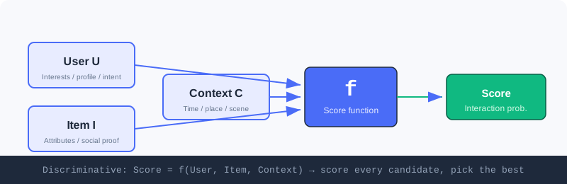
Discriminative recommendation integrates user features , item features , and context features to score each candidate item one by one, predicting the likelihood of a "valuable connection."
🧠 Mental Model: The Talent-Show Judge
Think of recommendation as a "talent-show judge." The stage is full of contestants (candidate items), and the judge (the model) scores each contestant individually, then hands out passes by score. The judge never "announces the list directly" — scoring is the judge's only job.
The Second Approach: Generative Recommendation
It fundamentally redefines the problem: instead of evaluating candidates one by one, the model directly "creates" the recommendation result based on its understanding of the user and context. The core is a generation function:
The model takes the user's historical interaction sequence and current context as input, and directly generates a sequence of recommended items through autoregressive decoding. This is like a friend who knows your taste — no need to comb through all the options; they just say "here's what you should watch next."
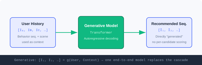
Generative recommendation takes the user's historical interactions and context as input, and directly outputs a sequence of recommended items through a generative model — no need to evaluate candidates one by one.
🤔 Why do both paradigms coexist? Discriminative recommendation is extremely mature and stable at "selecting the best from a finite candidate set"; generative recommendation has huge potential for "creating in an open space." The former asks "will the user like this item?", while the latter asks "what does the user want to see next?" — the former selects; the latter creates.
Four Stages of Capability Evolution
Looking at a longer timeline, recommendation algorithms show a clear trajectory of capability evolution, one that runs through both paradigms:
- Memorization on pure IDs — collaborative filtering treats items as opaque symbols, memorizing co-occurrence patterns like "people who watched A also watched B."
- Generalization through deep learning — deep networks generalize knowledge to unseen user—item combinations through feature crossing and sequence modeling, but items remain atomic IDs.
- Understanding through semantic IDs — when items are encoded as structured tokens carrying semantics, the system begins to truly "understand" content meaning; new items can be recommended without accumulating behavioral data.
- Reasoning with large models — instead of implicitly computing scores, the model explicitly analyzes intent, evaluates matches, and gives reasons, evolving from a "pattern matcher" into a "reasoner that can explain its decisions."
💡 Key Insight: These four stages do not linearly replace one another; they stack and coexist. In today's industrial systems, ID-based collaborative filtering remains a major retrieval channel, deep generalization supports every stage from retrieval to ranking, while semantic IDs and large-model reasoning are emerging at the frontier.
1.1.2 The Industrial Perspective: Two Technology Routes at Scale
Having understood the two basic paradigms, we immediately face a shared practical challenge: scale. A typical video platform has hundreds of millions of users and over a hundred million items, and recommendation must complete the entire process — from a massive item pool to a personalized list — within millisecond-level latency. If the page takes more than a few seconds to load, most users will leave.
⚠️ Warning: The core tension in recommender-system engineering is — how do we find the best result from a massive candidate pool within extremely limited time? The two paradigms offer fundamentally different answers.
The Discriminative Answer: A Multi-Stage Pipeline
The core difficulty of the discriminative paradigm is that computing a match score between every user and every item would instantly overwhelm even the strongest servers. Industry's answer is a staged funnel architecture, using the three-stage "retrieval—ranking—re-ranking" pipeline to progressively narrow the candidates, balancing efficiency and effectiveness.
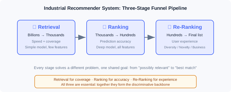
- ① Retrieval — quickly filter a few thousand possibly relevant candidates from the full item pool. Its motto is "better to over-include than to miss," prioritizing coverage over precision; models are simple and features are limited (e.g., using collaborative filtering to find similar users, or retrieving based on content similarity).
- ② Ranking — where the prediction function truly shines. It deploys the most complex deep models, fusing the full set of user/item/context features to compute a precise score for each candidate, maximizing prediction accuracy.
- ③ Re-ranking — the final optimization over the ranked list. It solves the problem that "the highest-scoring list ≠ the best-experience list": introducing diversity and novelty to avoid aesthetic fatigue when the top ten are all similar content, while handling business rules such as ads and operations.
💡 Key Insight: The essence of the three-stage pipeline is — use different strategies at different stages, progressively filtering from "possibly relevant" to "best match." Retrieval pursues coverage, ranking pursues precision, re-ranking pursues experience; all three are indispensable.
The Generative Answer: End-to-End Generation
Generative recommendation proposes a radically different approach: if the model can directly "generate" results, why do we still need multi-stage filtering? Generative recommendation treats the user's historical interaction sequence as "context," and directly decodes a sequence of item tokens through autoregressive models like Transformers — the entire process is completed end-to-end within a single unified model, with no retrieval/ranking/re-ranking cascade.
💡 Key Insight: The end-to-end architecture eliminates three core pain points of cascading architectures:
- Objective misalignment — retrieval optimizes relevance, ranking optimizes click-through rate, re-ranking optimizes diversity, each fighting its own war;
- Information loss — high-quality items filtered out at retrieval are forever invisible to later stages;
- Computational fragmentation — different stages use different models, making it hard to fully exploit modern GPU capacity.
The interactive demo below lets you experience the funnel process of "hundreds of millions → one list" firsthand:
Click "Next Step" or "Autoplay" to watch the candidate pool shrink step by step from hundreds of millions down to the final list of 10, and observe the different responsibilities each stage carries.
📊 Data Point: The two architectures currently develop in parallel in industry: the discriminative pipeline serves mature scenarios stably through "divide and conquer"; the generative architecture shows huge potential in frontier exploration through "end-to-end optimization."
1.1.3 The Macro Perspective: Building a Win-Win Ecosystem
Placing recommender systems in a broader view reveals a deeper question: is a technically perfect recommender system necessarily a truly excellent one? The answer is often no.
Consider the classic "accuracy trap": a user has just added a phone to their cart, and the system recommends that same phone to them. Click-through and conversion rates may approach 100%. By the metrics this is extremely "accurate," but what value does it create? Almost none — the user was going to buy it anyway; the recommendation merely repeats information the user already knows, with no incremental value.
💡 Key Insight: The ultimate goal of a recommender system is not to blindly maximize technical metrics, but to build a healthy ecosystem where all participants benefit long-term. The ecosystem rests on three pillars: users and creators, content, and the platform — the three are interdependent.
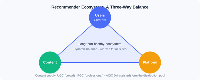
- Users and creators — sitting at the two ends of content consumption and supply. Users are the ultimate service target; the system should help them discover content they are "genuinely interested in but haven't yet encountered," rather than trapping them in an "ever-narrowing" filter bubble. Creators are the core of content supply; distribution capability directly determines their survival space and motivation. The supply side is shifting from primarily professional teams (PGC) toward ordinary users creating spontaneously (UGC) as the main body, with AI-assisted generation (AIGC) emerging as well, blurring the boundary between consumers and producers.
- Content — the medium connecting users and creators, and the true "atomic unit" of distribution. A healthy system must not only distribute popular content, but also continuously surface promising content, avoiding "concentration at the head, drowning of the long tail."
- The platform — the ecosystem's coordinator. It must optimize effectiveness — satisfaction and time spent — while also attending to long-term health (diversity, suppressing low quality, protecting creator motivation), sometimes sacrificing short-term metrics in exchange for long-term trust.
⚡ Pro Tip: A truly excellent recommender system is a delicate balancer — finding dynamic equilibrium among users, creators, content quality, and platform development. This requires designers to be not only technical experts, but also to possess an ecosystem mindset.
⚠️ Common Mistakes in 1.1
| # | Mistake | Example | Why It's Wrong | Fix |
|---|---|---|---|---|
| 1 | Equating recommendation with "ranking" | "A recommender system is just a click-through-rate prediction model" | Ranking is only one of three stages; retrieval comes before it and re-ranking after | Always understand recommendation through the full "retrieval→ranking→re-ranking" picture |
| 2 | Confusing the questions the two paradigms ask | Assuming generative recommendation also "scores every candidate" | The generative approach directly produces a sequence and does no per-candidate evaluation | Remember: discriminative selects, generative creates |
| 3 | Metrics-only thinking | Using a 100%-conversion "post-add-to-cart recommendation" to prove the system is excellent | No incremental value — falling into the accuracy trap | Ask: does the recommendation create value the user would not otherwise have gotten? |
| 4 | Ignoring the ecosystem's long-term nature | Mindlessly pushing clickbait for short-term watch time | Destroys trust and the creator ecosystem, collapsing in the long run | Evaluate trade-offs with the ecosystem triangle; dare to sacrifice short-term metrics |
Chapter Summary
📌 Key Takeaways
| Concept | Key Points | Why It Matters |
|---|---|---|
| Discriminative recommendation | , scoring and selecting among candidates one by one | The backbone of industrial recommendation — mature and stable |
| Generative recommendation | , directly generating a sequence | End-to-end with huge potential — the frontier direction |
| Three-stage pipeline | Retrieval (coverage) → ranking (precision) → re-ranking (experience) | Balances efficiency and effectiveness within millisecond latency |
| End-to-end generation | A single model replaces the multi-stage cascade | Solves objective misalignment, information loss, and compute fragmentation |
| Ecosystem triangle | Users/creators, content, platform | Look beyond metrics to understand the system's long-term value |
❓ FAQ
Q1: Which is better, discriminative or generative?
A: Neither is absolutely superior. Discriminative approaches are stable and efficient in mature scenarios; generative approaches have great potential in frontier exploration. The two currently develop in parallel in industry — choose based on your business stage.
Q2: Why not just show users the entire item pool and let them pick?
A: Among hundreds of millions of items, users will only look at a tiny fraction. The value of recommendation is precisely doing subtraction on the user's behalf within a space of hundreds of millions, and doing so within milliseconds — this is an engineering reality, not a design preference.
Q3: Why can the retrieval stage use "simple models"?
A: Retrieval's motto is "better to over-include than to miss"; its goal is coverage, not precision. The candidate set will be finely filtered by ranking afterward, so the retrieval side can trade lightweight models for speed.
🔗 Connections to Later Chapters
- 1.2 (book overview) maps this section's three perspectives onto the book's technology map, locating each chapter on the capability-evolution curve.
- 2.1–2.5 (retrieval) expands the concrete algorithm families of "retrieval" within the three stages.
- 3.1–3.5 (ranking) dives into the engineering implementation of the discriminative scoring function .
- 5.3 (evolution of the generative paradigm) echoes this section, systematically tracing the leap from discriminative to generative.
Practice Problems
Work through all problems in order — they get progressively harder. Each has a complete solution you can reveal after trying it yourself.
Problem 1.1.1 — Distinguishing Paradigms 🟢 Easy
Given the following two system descriptions, determine whether each is closer to the discriminative or generative paradigm, and explain why.
- (a) The system computes a "probability the user clicks" for each candidate ad, ranks by probability, and shows the top 5.
- (b) The system reads the user's last 20 plays and directly outputs "the 3 video IDs you might want to watch next."
💡 Solution (click to reveal)
Approach: Grasp the difference in the "questions asked" by the two paradigms — is it per-candidate scoring, or directly producing a sequence?
- (a) Discriminative: computing a click probability separately for each candidate ad and then ranking is exactly the "score one by one, select the best" of .
- (b) Generative: directly decoding a sequence of recommended IDs from the history, with no per-candidate evaluation, corresponds to .
Key points:
- Discriminative = candidates known, scored one by one; generative = directly "creates" a sequence.
- The key to judging is whether the system enumerates and evaluates every single candidate.
Problem 1.1.2 — Completing the Pipeline 🟢 Easy
A recommender system faces 100 million items and finally shows 10. Fill in the correct stage names in the brackets so it matches the industrial funnel:
Full item pool (100M) → [ ① ] → Candidates (~2000) → [ ② ] → Candidates (~200) → [ ③ ] → Final list (10 items)
💡 Solution (click to reveal)
Approach: Recall the "progression of responsibilities" in the three-stage funnel.
Full item pool (100M) → [ Retrieval ] → Candidates (~2000)
→ [ Ranking ] → Candidates (~200)
→ [ Re-ranking ] → Final list (10 items)
Key points:
- Retrieval pursues coverage, ranking pursues precision, re-ranking pursues experience (diversity/business).
- The scale shrinks level by level: 100M → thousands → hundreds → ten.
Problem 1.1.3 — Analyzing the Accuracy Trap 🟡 Medium
A news app finds that immediately recommending another "World Cup final" story to a user who just finished reading one achieves a 95% click-through rate. The product manager concludes the recommendation is "highly precise." Point out what's wrong with this conclusion, and propose a more reasonable evaluation perspective.
💡 Solution (click to reveal)
Approach: Use the "accuracy trap" framework to examine the mismatch between metrics and value.
Answer: The 95% click-through rate merely "repeats information the user already knows," creating no incremental value — the user would have opened follow-up stories on the same topic anyway. This falls into the accuracy trap: high metrics ≠ a good system.
More reasonable evaluation perspectives:
- Incremental value: does the recommendation lead the user to discover content they "would not have sought out on their own" (diversity, exploration)?
- Ecosystem health: is the system sinking into an "ever-narrowing" filter bubble that damages long-term retention?
- Multi-objective balance: beyond CTR, does the system also weigh long-term metrics like watch time, shares, and follows?
Key points:
- High technical metrics do not equal high user value.
- Evaluation should look beyond single-point accuracy to the long term and the ecosystem.
🏆 Challenge: Making the Design Trade-off
Suppose you need to build a recommender system from scratch for a new app with 10 million daily active users. Write an argument of no more than 150 words explaining: given sparse early-stage data and limited compute, why should you prioritize the discriminative three-stage pipeline over an end-to-end generative architecture? Also indicate which kinds of scenarios could pilot generative approaches once the business matures.
💡 Hint
Compare the two architectures across "data requirements, compute cost, interpretability, and iteration controllability"; in the mature stage, start generative pilots in components such as candidate generation/retrieval or re-ranking diversity.
Book Overview and Technology Map
📝 Before You Continue: Please read the three perspectives in 1.1 first. This chapter unfolds that "three-dimensional understanding" into a navigable technology map, helping you locate every chapter that follows.
Once you understand the core logic of recommender systems, the real challenge is turning that understanding into actionable technical solutions. Researchers and engineers have proposed hundreds of algorithms, and beginners often feel lost: how do these models relate to each other? Which one for which scenario? How do you assemble a complete system?
This chapter gives you a map. The book is organized along two main storylines — discriminative and generative — while also threading together the capability evolution from "memorization and generalization" to "understanding and reasoning."
After reading this chapter, you will be able to:
- State the logic behind the book's two halves and where each lands
- Map every chapter of the fundamentals half (Ch0–Ch4) onto the three-stage pipeline or frontier trends
- Explain why "retrieval → ranking → re-ranking" is the organizing thread of the discriminative storyline
- Anticipate how the generative storyline will unfold in later versions (Ch5–Ch10)
- Complete 4 leveled practice problems to verify your grasp of the technology map
1.2.0 One Map, Two Storylines
The book's organization can be summarized in one diagram: the horizontal axis is time/capability evolution (from pure-ID memorization to LLM reasoning), and the vertical axis is the two paradigm storylines (discriminative vs generative).
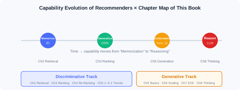
- First half: industrial practice of discriminative recommendation — progressively deepening along the "retrieval → ranking → re-ranking" pipeline; the main battlefield of memorization and generalization capabilities.
- Second half: the technology landscape of generative recommendation — starting from the foundational paradigm, through Scaling Laws, end-to-end modeling, and reasoning capability to diffusion models; the exploration ground of understanding and reasoning capabilities.
💡 Key Insight: The two storylines are not isolated. Generative architectures often "end-to-end-ify" mature discriminative modules; meanwhile, discriminative techniques such as semantic IDs and feature crossing provide the representational foundation for generative approaches.
1.2.1 First Half: Industrial Practice of Discriminative Recommendation (Covered in This Edition)
This edition (the fundamentals half) fully covers the first half plus the bridging trends chapter — 5 parts in total:
| Part | Theme | Position in the Pipeline | Core Content |
|---|---|---|---|
| Part 1 | Introduction and Overview | — | Two paradigms, three-stage funnel, ecosystem triangle, feature and Embedding basics |
| Part 2 | Fast Candidate Retrieval | ① Retrieval | Collaborative filtering / vector retrieval / two-tower / sequence retrieval / streaming index |
| Part 3 | Accurate Preference Prediction | ② Ranking | Wide&Deep / feature crossing / sequence modeling / multi-objective / multi-scenario |
| Part 4 | Re-ranking and Diversity Modeling | ③ Re-ranking | Greedy re-ranking (MMR/DPP) / personalized re-ranking (PRM) |
| Part 5 | Frontier Trends | Cross-stage | Model debiasing / cold start / evolution of the generative paradigm |
Retrieval: From 100 Million to Thousands (Part 2)
Retrieval is the pipeline's starting point: it must filter from hundreds of millions of items down to thousands of candidates within milliseconds. Its technical evolution unfolds across five sections:
- Collaborative filtering — the classic starting point: from ItemCF's item similarity, through Swing's industrial optimization and UserCF's user perspective, to matrix factorization mapping users/items into latent vectors, pioneering vectorization.
- I2I vector retrieval — transplanting Word2Vec's sequence-modeling ideas into recommendation: from Item2Vec's direct transfer, to EGES fusing side attributes, to Airbnb embedding business objectives into sequence construction.
- Two-tower models (U2I) — encoding users and items separately as vectors, represented by FM, DSSM, and YoutubeDNN, enabling efficient vector retrieval.
- Sequence retrieval — attending to the temporal information earlier methods ignored: MIND uses multiple vectors to represent diverse interests; SDM separates long- and short-term preferences and fuses them dynamically with gating.
- Streaming index retrieval — stepping outside model-internal compression: Trinity uses clustering statistics to preserve full historical interests; Streaming VQ lets the index structure adapt to data distribution in real time.
Ranking: From Thousands to Hundreds (Part 3)
Ranking scores thousands of candidates precisely — the main battlefield of deep generalization:
- Wide & Deep — jointly training a linear model and a deep network, establishing the foundational "memorization + generalization" framework.
- Feature crossing — from FM's second-order crossing, through DeepFM and xDeepFM, toward automatic high-order crossing.
- Sequence modeling — DIN uses attention to dynamically activate history based on the candidate; DIEN explicitly models the temporal evolution of interests.
- Multi-objective / multi-scenario — MMoE and ESMM balance multiple objectives; multi-tower and dynamic weights adapt to cross-scenario differences.
Re-ranking: From Hundreds to One Screen (Part 4)
Ranking output is often highly homogeneous; re-ranking optimizes the whole-list experience while preserving relevance:
- Greedy re-ranking — MMR linearly combines relevance and diversity; DPP uses a determinant framework to control diversity more precisely.
- Personalized re-ranking — PRM uses a Transformer to model mutual influence among items, achieving end-to-end personalized list generation.
1.2.2 Preview of the Second Half: Generative Recommendation (Covered in Later Versions, Ch5–Ch10)
To help you build a complete picture, here is a brief preview of the second half, so you know where the road leads after this edition:
| Chapter | Theme | In One Sentence |
|---|---|---|
| Ch5 | Generative foundations | Transformer / diffusion models / LLM workflows / item tokenization (semantic IDs) |
| Ch6 | Scaling Law architectures | HSTU turns per-candidate scoring into user-level sequence modeling; RankMixer builds a hardware-aware unified architecture |
| Ch7 | End-to-end generation | OneRec (recommendation) / OneSug·OneSearch (search) / EGA (ads) replace the pipeline with a single model |
| Ch8 | Recommenders that think | Semantic alignment (LC-Rec) → reasoning activation (OneRec-Think) → autonomous reasoning (RecZero) |
| Ch9 | Diffusion-model recommendation | DiffuASR data augmentation / AsymDiffRec·DMSG feature and diversity optimization |
| Ch10 | Production-grade project | Full-stack movie recommendation: offline training + online serving + frontend + Docker deployment |
📝 Note: This edition focuses on the fundamentals half (Ch0–Ch4). The second half will be continued in later editions under the same book-writer conventions.
⚠️ Common Mistakes in 1.2
| # | Mistake | Example | Why It's Wrong | Fix |
|---|---|---|---|---|
| 1 | Treating chapters as isolated algorithms | "This chapter covers DIN, the next covers DIEN — they're unrelated" | Chapters are consecutive stages on one pipeline; each chapter's output feeds the next | Always understand each chapter through its "pipeline position" |
| 2 | Memorizing model names without motivations | Reciting FM/DeepFM but unable to explain why high-order crossing is needed | Models exist to solve specific limitations; learning without motivation doesn't stick | For every model, first ask "what shortcoming of the previous method does it solve" |
| 3 | Mistakenly believing generative replaces discriminative | "Now that I've studied generative, I can skip the first half" | The two develop in parallel; generative approaches often build on discriminative representations | Treat the two storylines as complementary, not substitutes |
Chapter Summary
📌 Key Takeaways
| Concept | Key Points | Why It Matters |
|---|---|---|
| Two storylines | Discriminative (first half) / generative (second half) | The book's organizational skeleton — it determines how you categorize every model |
| Three-stage thread | Retrieval→ranking→re-ranking runs through the first half | Understand each chapter's position in the pipeline |
| Capability evolution | Memorization→generalization→understanding→reasoning | Explains why the technology keeps iterating rather than simply being replaced |
| Edition boundary | Covers Ch0–Ch4 (fundamentals half) | Clarifies this edition's scope and avoids misplaced expectations |
❓ FAQ
Q1: Why does the fundamentals half stop at Ch4 instead of including Ch5's generative content?
A: Ch5 is the cornerstone of the generative storyline, and its conceptual density rises sharply (semantic IDs, Transformers, diffusion models). First solidifying the industrial practice of discriminative recommendation, then moving into generative, makes for steadier learning.
Q2: Must retrieval, ranking, and re-ranking all use deep learning?
A: No. Retrieval often uses lightweight methods (collaborative filtering, two-tower); only ranking deploys the most complex deep models; re-ranking can use rules or lightweight models. Complexity increases as candidates shrink.
Q3: What order should I read in?
A: Strictly in Part 1→5 order. Later chapters often presuppose earlier ones (e.g., sequence modeling builds on feature crossing).
🔗 Connections to Later Chapters
- Part 2 Retrieval (Ch2.1–2.5) expands this chapter's "Retrieval: from 100 million to thousands" into five algorithm families.
- Part 3 Ranking (Ch3.1–3.5) dives into the industrial implementation of the discriminative scoring function .
- Part 4 Re-ranking (Ch4.1–4.2) wraps up the three-stage pipeline and connects to the trends chapter.
- Part 5 Trends (Ch5.1–5.3) bridges with "debiasing / cold start / generative," pointing toward the second half in later editions.
Practice Problems
Problem 1.2.1 — Locating Chapters 🟢 Easy
Place each of the following algorithms into its correct position in the pipeline (write the corresponding Part/chapter): (a) DPP re-ranking (b) YoutubeDNN two-tower (c) DeepFM feature crossing (d) Swing collaborative filtering
💡 Solution (click to reveal)
Approach: Recall the three stages and the representative models of each.
| Algorithm | Position |
|---|---|
| (a) DPP re-ranking | Part 4 Re-ranking (Ch4.1 greedy re-ranking) |
| (b) YoutubeDNN two-tower | Part 2 Retrieval (Ch2.3 two-tower U2I) |
| (c) DeepFM feature crossing | Part 3 Ranking (Ch3.2 feature crossing) |
| (d) Swing collaborative filtering | Part 2 Retrieval (Ch2.1 collaborative filtering) |
Key points:
- Retrieval-side methods are lightweight and coverage-oriented; ranking-side methods deploy complex deep models.
- Re-ranking happens after ranking and optimizes list-level experience.
Problem 1.2.2 — Classifying Capability Stages 🟢 Easy
Classify the following techniques into one of the four capability stages — "memorization / generalization / understanding / reasoning": (a) Collaborative-filtering co-occurrence (b) Deep feature crossing (c) Semantic IDs (RQ-VAE) (d) OneRec-Think explicit reasoning
💡 Solution (click to reveal)
Approach: Check against the capability-evolution curve.
- (a) Memorization (pure-ID co-occurrence)
- (b) Generalization (deep networks extrapolating to unseen combinations)
- (c) Understanding (items encoded as semantics-carrying tokens)
- (d) Reasoning (the model explicitly analyzes intent and gives reasons)
Key points:
- The four stages stack rather than replace; the same evolution curve threads the whole book.
Problem 1.2.3 — Probing Motivations 🟡 Medium
Why did "feature crossing" evolve from FM's second order to xDeepFM's automatic high order? Use a concrete example to illustrate: what kind of pattern would second-order crossing alone miss?
💡 Solution (click to reveal)
Approach: Start from "what limitation is the model trying to solve." FM's second-order crossing only models pairwise feature combinations (e.g., gender×category). But in real businesses, value often comes from higher-order interactions — for example, the three-way combination "tier-1 city × young female × beauty category" is what triggers strong interest.
With only second-order crossing, the model cannot explicitly capture such third-order (and higher) synergy signals; it can only approximate them implicitly, limiting expressiveness. xDeepFM and its kin use vectors/neural networks to learn arbitrary-order crossings automatically, escaping manual feature engineering and covering high-order patterns.
Key points:
- Second-order crossing = pairwise combinations; high-order crossing = multi-feature joint patterns.
- Evolution motive: insufficient expressiveness → automated high-order interaction.
🏆 Challenge: Designing Your Reading Route
Suppose a colleague "only knows SQL and basic logistic regression, has never touched deep learning," but urgently needs to get up to speed on your company's recommendation ranking module within two weeks. Based on this chapter's technology map, design a two-week learning route for them (listing which chapters to read per day/phase, what to skip, and why), and explain your reasoning (within 150 words).
💡 Hint
Prioritize the "pipeline mainline": Part1 → Part2 retrieval → Part3 ranking (Wide&Deep, feature crossing, sequence modeling); re-ranking and trends can be deferred; generative (Ch5+) can be skipped for now. The reasoning: the ranking module depends most on Part3, and the deep-learning foundation can be approached smoothly through Wide&Deep.
Feature and Embedding Basics
📝 Before You Continue: Please first read the user—item—context triple in 1.1 and the technology map in 1.2. You need to be able to read basic C++ and know that a hash function can map a string to an integer deterministically; no machine learning background is required.
What a recommender system ultimately processes is not an abstract "user interest," but a set of concrete fields: gender=male, city=Beijing, ad_id=10001, estimated_ctr=0.073. Business code understands these fields, but a neural network only accepts numeric tensors. A bridge is missing between the two.
That bridge is feature processing. It turns raw business fields into slotId + featureSign + value, and the model service then looks up the meaningless IDs to obtain learnable Embedding vectors. This pipeline looks like nothing more than a data-format conversion, yet it determines what the model can see, how it generalizes, and whether training and online serving stay consistent.
1.3.0 From Business Fields to Model Input
A ranking request typically carries four kinds of information at once:
| Category | Typical Fields | Question Answered |
|---|---|---|
| User information | User ID, gender, age, city | Who is this person? What are their long-term preferences? |
| Item information | Ad ID, video ID, category, author | What is the current candidate? |
| Context information | Time, network, device, candidate position | In what situation does this request occur? |
| Continuous values | Estimated CTR, eCPM, quality score, duration | Exactly how strong is a given signal? |
All of this model-usable information is collectively called a feature. But raw values cannot be fed into the model as-is: strings cannot participate in matrix multiplication; the numeric magnitude of a business ID carries no semantics; and the scales of different continuous values can differ by a factor of billions.
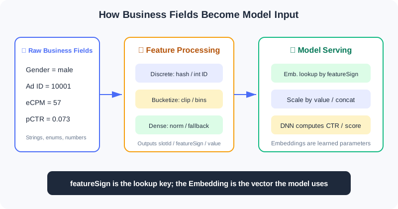
The figure above shows the full division of responsibilities: the business service generates features, while the model service looks up Embeddings, combines features, and performs the network computation. The two are connected by a stable feature protocol.
💡 Key Insight: Feature processing is not just "turning things into numbers." It must simultaneously preserve categorical identity, numeric magnitude, and engineering stability, while ensuring that offline training and online prediction see the same representation.
1.3.1 The Triple: slotId / featureSign / value
Industrial systems typically organize a feature as the following record:
struct FeatureInfo {
int slotId; // which field or feature group this feature belongs to
int64_t featureSign; // lookup key for the specific value
float value; // numeric value or weight
};
Each of the three fields manages one thing:
| Field | Meaning | Library Analogy |
|---|---|---|
slotId | What type of feature this is | Which shelf |
featureSign | The ID of this specific value | The index number of a book on that shelf |
value | The numeric value or weight for this occurrence | How strongly the book is used this time |
For example, when the user's gender is male, it can be expressed as:
FeatureInfo sex_feature{
.slotId = SEX,
.featureSign = gen_feasign_string(SEX, "male"),
.value = 1.0F
};
This reads as: "Go to the SEX shelf, find the entry for the value 'male', with weight 1.0 for this occurrence."
Continuous features divide the labor differently. If the estimated click-through rate is 0.073:
FeatureInfo ctr_feature{
.slotId = AD_ETR_DENSE,
.featureSign = 1,
.value = 0.073F
};
Here featureSign=1 is just a fixed placeholder; the real information lives in value. Keep this contrast in mind:
| Feature Representation | What Goes in featureSign | What Goes in value | Where the Information Lives |
|---|---|---|---|
| Sparse / bucketed | The ID of the category or bucket | Usually 1.0 | featureSign |
| Dense continuous | A fixed key, commonly 1 | The true normalized value | value |
⚠️ Warning:
featureSignshould be treated as an opaque 64-bit key. If it is generated asuint64_tand then stored in anint64_t, values with the highest bit set will appear negative under common two's-complement implementations. As long as downstream lookups use the same bit pattern, this is usually harmless — but never perform magnitude comparisons,abs(), or signed modulo on it.
1.3.2 How featureSign Is Generated
One common design places slotId in the high 32 bits and the ID of the specific value in the low 32 bits:
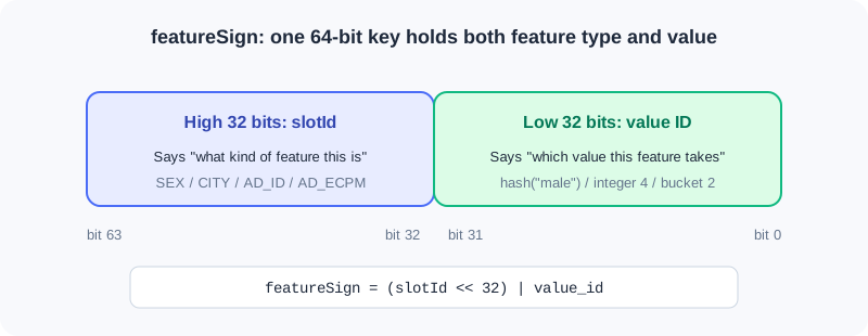
This way, even if the low-bit IDs of two fields happen to coincide, as long as their slotIds differ, the final keys still differ.
String Values: Hash First, Then Combine
static uint64_t gen_feasign_string(
uint64_t slot_id,
const std::string& value) {
const uint32_t value_hash = gen_hash_new(value.data(), value.size());
const uint64_t slot_bits = (slot_id << 32) & 0xffffffff00000000ULL;
return slot_bits | value_hash;
}
This code works in three steps:
gen_hash_newdeterministically maps the string to a 32-bit integer.slot_id << 32moves the feature type into the high 32 bits.- A bitwise OR
|combines the high-bit type and the low-bit value into one key.
For example, even if the low-bit hashes of SEX=male and AGE_BUCKET=20 both equal 111, the final keys remain [SEX][111] and [AGE_BUCKET][111] respectively. Slot segmentation isolates different fields from each other.
💡 Key Insight:
featureSignworks like "class number + student number." The student number only distinguishes students within a class; the class number in the high bits keeps identical student numbers from different classes from colliding.
Integer Values: Encode Directly When Possible, Skip the Hash
If the value is already a small integer — for example network type 4, weekday 2, or bucket ID 7 — it can go directly into the low 32 bits:
static uint64_t gen_feasign_int32(
uint64_t slot_id,
uint32_t value) {
const uint64_t slot_bits = (slot_id << 32) & 0xffffffff00000000ULL;
return slot_bits | value;
}
As long as the value can be fully represented by a 32-bit unsigned integer, this encoding introduces no extra hash collisions. Therefore, small enums and bucket IDs should prefer the integer version.
Hash Collisions Are a Trade-off, Not an Error
Once strings are compressed into a 32-bit space, collisions are unavoidable. The low 32 bits offer only positions; by the birthday paradox, once a slot has about 77,000 distinct values, the probability of at least one collision exceeds 50%.
| Example Slot | Cardinality | Collision Impact |
|---|---|---|
SEX | Negligible | |
CITY | Usually negligible | |
AD_ID | A few collisions appear | |
GUID | Massive collisions are unavoidable |
After two distinct values collide, they share one Embedding, and the model can no longer tell them apart. So why do industrial systems still commonly use this Feature Hashing? Because it buys stateless, scalable feature generation: no giant string vocabulary needs to be maintained, and new values get a key immediately.
Analysis:
- Benefit: No central vocabulary needed; new values are handled naturally; online services scale horizontally.
- Cost: Some semantic confusion; the original value cannot be recovered from the key; high-cardinality features are harder to debug.
- Mitigation: Enlarge the hash space, use double hashing, filter low-frequency values, or maintain an independent vocabulary for critical high-cardinality slots.
1.3.3 Why Embeddings Are Needed
This is the most easily confused — and most critical — point of the chapter:
💡 Key Insight:
featureSignis the key for looking up an Embedding; it is not the Embedding itself. It is responsible for stably indicating "which category this is," but not for expressing how this category relates to other categories.
The difference between the two:
| Object | Example | Trained? | Essence |
|---|---|---|---|
featureSign | 500111 | No | A stable, discrete index key |
| Embedding | [0.12, -0.03, 0.88, 0.21] | Yes | Vector parameters learned by the model from data |
| Embedding Table | key → vector | Yes | A parameter table that stores and updates vectors by key |
From One-Hot to Embedding
Suppose CITY has only three values: Beijing, Shanghai, and Shenzhen. The most direct encoding is One-Hot:
Beijing -> [1, 0, 0]
Shanghai -> [0, 1, 0]
Shenzhen -> [0, 0, 1]
One-Hot has two properties: first, it never falsely creates magnitude relations; second, all categories are equidistant from each other. But when an ad ID has 10 million values, a single sample must logically occupy a 10-million-dimensional space, with only one position in the vector set to 1. Feeding such ultra-high-dimensional sparse vectors directly into the network makes both parameter count and computation prohibitive.
The Embedding layer can be viewed as a large matrix . Multiplying a One-Hot vector by the matrix is essentially selecting one row from :
So in practice you never actually construct the One-Hot. Just pass in the featureSign of the category and directly look up . This saves computation and lets the model, through training, pull categories with similar behavior into nearby regions of the vector space.
Why You Can't Use featureSign Directly as an Embedding
Suppose there are three ads:
Sneaker ad -> featureSign = 105
Basketball ad -> featureSign = 980001
Baby formula -> featureSign = 106
If the sign were used directly as a scalar input, the model would be handed absurd geometric relationships: the distance between sneakers 105 and baby formula 106 is only 1, while the semantically closer basketball ad 980001 is nearly a million away. This distance is determined entirely by chance of numbering or hashing, and represents nothing about behavioral similarity.
Using the sign directly has four further problems:
- Spurious ordering.
500222 > 500111does not mean one category is "bigger" or "better." - Spurious distances. Two hash values being close does not mean the two categories are similar; being far apart does not mean dissimilar.
- No way to learn category semantics. The sign is a fixed integer; it will never move toward "more like basketball" or "more like sneakers" during backpropagation.
- Numeric precision risk. If a 64-bit sign is converted to
float32, beyond many adjacent integers can no longer be distinguished exactly, and different keys may be rounded to the same float.
An Embedding instead provides a set of trainable parameters for each key. If users who watch basketball content often click sneaker ads, training will gradually pull the two categories' vectors together; the baby-formula vector may end up in a different region. Distances between categories are learned from data, not dictated by hash values.
⚠️ Warning: "Converting the sign into 8 binary digits, splitting it by decimal digit, or normalizing it" is still not an Embedding. These operations merely expose an arbitrary ID in another way and cannot produce learnable category semantics. The correct approach is to treat the sign as an index and look up an independent, trainable vector.
A Complete Lookup
Suppose SEX=male generates featureSign=500111, and the Embedding table currently stores:
E[500111] = [ 0.12, -0.03, 0.45]
E[500222] = [-0.21, 0.34, 0.08]
During the forward pass, the model uses 500111 to look up the first row [0.12, -0.03, 0.45]. If this prediction's error back-propagates to this feature, only E[500111] and the related network parameters are updated — the integer 500111 itself is never modified.
This shows the strict separation of responsibilities:
featureSign: stably locates parameters; unchanged before and after training
Embedding: carries learnable semantics; continuously updated during training
Why the Same Value Shares One Embedding
Two users who both have SEX=male generate the same featureSign and therefore look up the same Embedding. This does not make the two users indistinguishable, because the model sees a combination of many slots:
| User | Gender | Age Bucket | City | GUID |
|---|---|---|---|---|
| A | Male | 20–24 | Beijing | abc |
| B | Male | 35–39 | Shenzhen | xyz |
Sharing actually brings generalization: the samples of all male users jointly update the "male" parameter, while other features — age, city, identity — continue to preserve individual differences.
What Determines the Embedding Dimension
The dimension is not decided by the C++ feature-generation code, but by the model configuration, usually set per slot or per feature group:
| Slot | Possible Cardinality | Typical Dimension Guidance |
|---|---|---|
SEX | 3 | 2–4 dimensions usually suffice |
CITY | Start experimenting from 8 | |
AD_ID | Commonly a trade-off within 8–32 | |
GUID | Dimension times cardinality becomes a memory black hole — be careful |
The larger the dimension, the stronger the representational capacity, but the higher the memory, communication, and compute costs; with insufficient data it is also more prone to overfitting. It is a hyperparameter balancing model capacity against system cost — not "cardinality grows, so keep adding dimensions."
1.3.4 How Sparse and Dense Features Are Encoded
Both sparse and dense features fit into slotId + featureSign + value, but the field that "actually carries the information" is completely different on the two paths:
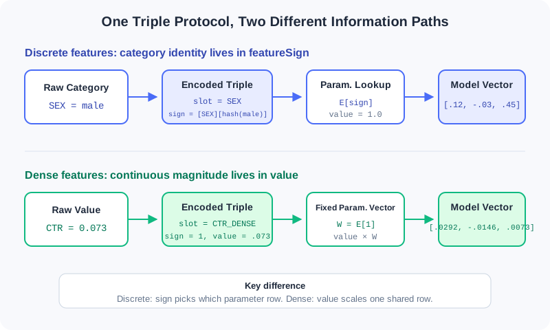
A sparse feature uses featureSign to select "which row of parameters"; a dense feature usually fixes the sign and uses value to determine "how much to scale the same set of parameters."
| Aspect | Sparse Features (Categorical) | Dense Features (Continuous / Numerical) |
|---|---|---|
| Question answered | Which category is it? | Exactly how much? |
| Typical values | Beijing, male, ad 10001, network type 4 | CTR 0.073, duration 3600 seconds, amount 57 yuan |
| Arithmetic relations | Magnitude and distance usually meaningless | Addition/subtraction, magnitude, and differences usually meaningful |
| Location of information | featureSign | value |
| Typical model handling | Look up Embedding by sign | Fed in directly or projected into a vector |
Sparse Features: Encoding "Which Category"
Sparse features take values from a finite or enumerable set. Their numeric form is mere identity and should not be interpreted as continuous magnitude. Network type 4 does not mean it is twice network type 2; ad ID 10002 is not "better" than 10001.
A sparse feature typically goes through five steps:
- Normalize the raw value. Unify encoding, casing, whitespace, and missing values — for example, map an empty city to
__UNKNOWN__. - Choose the slot.
CITY,SEX, andAD_IDeach have their ownslotId. - Generate the sign. Strings are hashed first; small integers can be encoded directly into the low 32 bits.
- Set the weight. Single-valued categories usually use
value=1.0. - Look up the Embedding. The model uses the sign to select one row in the parameter table.
Example 1: String Category SEX=male
Suppose SEX has slotId=12, and assume hash("male")=0x3A91F20B. Then:
High 32 bits: slotId = 12 -> 0x0000000C00000000
Low 32 bits: hash("male") -> 0x000000003A91F20B
Final sign -> 0x0000000C3A91F20B
The business service generates:
const std::string normalized_sex = user.sex.empty()
? "__UNKNOWN__"
: user.sex;
features.emplace_back(
SEX,
gen_feasign_string(SEX, normalized_sex),
1.0F);
The model-side handling can be written as:
embedding = E_SEX[0x0000000C3A91F20B]
= [0.12, -0.03, 0.45]
output = 1.0 × embedding
= [0.12, -0.03, 0.45]
Here value=1.0 merely states "this category occurs in this instance." What actually distinguishes male, female, and unknown are the different signs, and the Embeddings each of them maps to.
Example 2: Integer Enum APN_TYPE=4
The network type is already a small integer; there is no need to convert it to a string and hash it first:
features.emplace_back(
APN_TYPE,
gen_feasign_int32(APN_TYPE, 4),
1.0F);
This generates [APN_TYPE][4]. Compared with the string version, it is more intuitive and introduces no additional 32-bit hash collisions.
How Multi-Value Sparse Features Are Handled
"User interest tags" may simultaneously include basketball, running, photography. In this case one slot yields multiple signs:
[INTEREST][hash(basketball)] value=1.0
[INTEREST][hash(running)] value=1.0
[INTEREST][hash(photography)] value=1.0
After looking up the three Embeddings, the model usually applies sum, mean, weighted pooling, or attention-based aggregation. If the number of tags varies a lot, mean avoids the bias of "more tags, larger vector norm"; if different tags carry different importance, you can put business weights into value.
Analysis:
- Strengths: No spurious ordering; parameters learned independently per category; behavioral patterns shared through the vector space.
- Costs: High-cardinality slots produce large tables; low-frequency categories get under-trained vectors.
- Key check: The same business value must produce exactly the same sign offline and online.
Dense Features: Encoding "Exactly How Much"
Dense features are numbers with continuous magnitude semantics. CTR=0.08 is genuinely larger than CTR=0.02; watching 100 seconds is usually longer than watching 10. Encoding should preserve this numeric relationship rather than creating a separate Embedding for every decimal value.
Dense features have two common implementations across frameworks:
- Direct scalar input. Concatenate the normalized with other vectors and feed it into the MLP.
- Unified slot protocol. Use a fixed
featureSign=1to look up a parameter vector , and output .
This chapter's engineering uses the second. It is mathematically equivalent to projecting a one-dimensional scalar into dimensions through a bias-free linear layer:
A dense feature typically goes through four steps:
- Validate and fall back. Handle missing values,
NaN,inf, and illegal negatives. - Transform and normalize. Depending on the distribution, use it directly,
log1p, Min-Max, Z-Score, or quantile transformation. - Fix the sign. The slot uniformly uses
featureSign=1, meaning only one set of projection parameters is needed. - Put the number into value.
value=x; the model computesx × E[1].
Example 1: Already-Normalized CTR=0.073
CTR itself lies in , so it can be used directly at first:
double ctr = ad.estimated_ctr;
if (!std::isfinite(ctr)) ctr = 0.0;
ctr = std::clamp(ctr, 0.0, 1.0);
features.emplace_back(
AD_ETR_DENSE,
1,
static_cast<float>(ctr));
Suppose this slot's fixed parameter vector is:
W = E_AD_ETR_DENSE[1] = [0.40, -0.20, 0.10]
Then the vector this sample passes to the upper network is:
0.073 × W = [0.0292, -0.0146, 0.0073]
Another sample with CTR=0.20 still looks up the same , but the output becomes [0.08, -0.04, 0.02]. The dense path thus preserves the continuous relationship "0.20 is larger than 0.073."
Example 2: Long-Tailed Watch Duration watch_seconds=3600
Duration usually follows a long-tailed distribution. Putting 3600 directly into value would make its magnitude dwarf features like CTR. You can apply log1p first:
double seconds = watch_seconds;
if (!std::isfinite(seconds) || seconds < 0.0) seconds = 0.0;
seconds = std::min(seconds, 86400.0); // cap the top at 24 hours
const float encoded = static_cast<float>(std::log1p(seconds));
features.emplace_back(WATCH_TIME_DENSE, 1, encoded);
3600 seconds is compressed to about 8.19, preserving the monotonic "longer" relation while reducing the dominance of extreme values over gradients and other features.
📝 Note: The
E[1]in a dense slot is sometimes colloquially called an "Embedding" too, but its role differs from a sparse categorical Embedding. A sparse Embedding is "one row per category"; a dense slot has only a single fixed row, essentially a set of learnable projection weights.
⚠️ Warning: Dense features cannot be stuffed into
valueunchecked. Large-magnitude values like timestamps, amounts, and counts will drown out other features and amplify gradients. Scale compression and outlier handling must come first.
Common processing methods:
| Method | Form | Suitable Scenarios |
|---|---|---|
log1p | Long-tailed positive values: counts, durations, amounts, eCPM | |
| Min-Max | Stable and known value range | |
| Z-Score | Approximately normal distribution | |
| Quantile normalization | Map to the empirical CDF | Irregular distributions with many outliers |
| Use directly | Unchanged | Already in , e.g., probability values |
Whichever method you choose, you must specify fallback rules for NaN, inf, missing values, and abnormal negatives. The min/max/\mu/\sigma values, quantile points, and truncation thresholds must also be shared between offline training and online serving.
Bucketing: Which Interval Does It Fall In
Bucketed features first cut a continuous value into intervals, then treat the bucket ID as a category:
static uint32_t cut_bucket(double value, uint32_t width) {
return static_cast<uint32_t>(value / width);
}
If eCPM=57 and the bucket width is 20, the bucket ID is 2. The final expression is [AD_ECPM][2] with value=1.0.
This is not a dense feature. It expresses "which interval it falls in"; each bucket has its own Embedding, so non-monotonic interval effects can be learned.
The raw cut_bucket still has three engineering traps:
- Negative values: values in may silently truncate into bucket 0; more negative values may exceed the representable range when converted to an unsigned integer — do not rely on that result.
NaN/inf: converting to an integer has no usable semantics and may trigger undefined behavior.- Zero bucket width: division by zero yields an invalid result.
A safer implementation should validate parameters first, clamp abnormal values, and set a top bucket:
#include <algorithm>
#include <cmath>
#include <cstdint>
#include <stdexcept>
uint32_t safe_cut_bucket(
double value,
double width,
uint32_t max_bucket) {
if (!std::isfinite(width) || width <= 0.0) {
throw std::invalid_argument("bucket width must be positive");
}
if (!std::isfinite(value) || value < 0.0) {
value = 0.0; // ← KEY LINE: unified fallback for abnormal inputs
}
const double raw_bucket = std::floor(value / width);
const double capped = std::min(raw_bucket,
static_cast<double>(max_bucket));
return static_cast<uint32_t>(capped);
}
Analysis:
- Equal-width bucketing: simple to implement, but long-tailed distributions often cram most samples into the first few buckets.
- Equal-frequency bucketing: more balanced samples per bucket, but depends on stable quantile statistics.
- Logarithmic bucketing: suits positive values spanning several orders of magnitude, balancing head and tail.
- Top-bucket capping: prevents extreme values from creating hordes of sparse buckets that appear only once or twice.
Why Bucketing and Dense Are Often Used Together
| Aspect | Bucketed Sparse | Dense Continuous |
|---|---|---|
featureSign | Bucket ID | Fixed key |
value | 1.0 | The true normalized value |
| Number of parameter rows | One per bucket | One for the whole slot |
| Good at | Non-linearity, interval effects | Exact magnitude, continuous variation |
| Limitations | No resolution within a bucket; discontinuous boundaries | A single linear scaling struggles with complex non-monotonic relations |
Using both is not pointless duplication. Bucketing tells the model "which interval it's in"; dense tells the model "exactly how much." They express the same business quantity from different angles.
1.3.5 The Embedding Table and Engineering Boundaries
Table Size Is Determined by the Number of Unique Values
The main memory of an Embedding table can be roughly estimated as:
where is the number of unique featureSigns in that slot, and is the Embedding dimension. Real systems must also account for hash-table metadata, keys, pointers, and optimizer states; optimizers like Adam may additionally store one or two same-sized copies of state.
Table size does not directly depend on request volume. If a billion users have only three genders, the SEX slot still needs only a handful of entries; but GUID is nearly "one value per user," so its scale grows with the user base.
Admission, Eviction, and OOV
High-cardinality slots keep producing new keys, so production systems must constrain table growth:
| Mechanism | Typical Strategy | Problem Solved |
|---|---|---|
| Admission | Create an entry only after the count reaches a threshold | Filters one-off noise and ultra-long-tail values |
| Eviction | Delete after being absent for several consecutive days | Cleans up inactive users and offline ads |
| OOV | Zero vector, default bucket, or deferred entry creation | Handles new keys not yet in the table |
"What happens when a key is not found" must be confirmed before adding any new feature. If downstream defaults to "randomly initialize and write immediately," a high-cardinality feature can bloat the parameter table in a short time; if a zero vector is returned, that feature contributes nothing during cold start, and the model must rely on other generalizable features.
How Embeddings Are Trained
Embeddings are part of the recommendation model, trained jointly with the upper network:
- The forward pass looks up vectors by
featureSign. - Multiple vectors are concatenated or pooled with dense features.
- The DNN outputs click-through rate, conversion rate, or a ranking score.
- Prediction error back-propagates, updating both the Embeddings and the network parameters.
Only keys covered by training samples receive effective updates. Long-tail features that appear only once or twice have vectors close to their random initialization — occupying memory while injecting noise. This is exactly why frequency-based admission exists.
Offline/Online Consistency
This is the most hidden and most common source of incidents in feature engineering. Training samples and online requests must be strictly aligned:
- Hash algorithm, seeds, and string encoding;
slotIdenum values and candidate-position offsets;- Bucket boundaries, bucket widths, and top buckets;
- Normalization statistics;
- Missing-value, outlier, and casing rules;
- String
trim, concatenation order, and separators.
These bugs often do not crash. The service still returns scores, monitoring may be all green — the model just looks up "wrong but legal" parameters, and online performance quietly degrades.
⚡ Pro Tip: Treat changing the hash, changing slots, or changing bucket boundaries as "swapping the model," not a routine code hotfix. Prioritize sharing one feature library between offline and online; before launch, sample real requests and compare the triples generated on both sides field by field.
1.3.6 Complete Case Study: Adding an eCPM Feature to Ads
Suppose the business already has ad.ecpm, and we want to preserve both its exact magnitude and its non-linear interval effects. The sound approach is to create two different slots:
#include <algorithm>
#include <cmath>
#include <cstdint>
#include <vector>
struct FeatureInfo {
uint32_t slot_id;
uint64_t feature_sign;
float value;
};
enum Slot : uint32_t {
AD_ECPM_BUCKET = 101,
AD_ECPM_DENSE = 102
};
uint64_t make_int_sign(uint32_t slot_id, uint32_t value_id) {
return (static_cast<uint64_t>(slot_id) << 32) | value_id;
}
uint32_t safe_bucket(double value,
double width,
uint32_t max_bucket) {
if (!std::isfinite(value) || value < 0.0) value = 0.0;
if (!std::isfinite(width) || width <= 0.0) return 0;
const double bucket = std::floor(value / width);
return static_cast<uint32_t>(
std::min(bucket, static_cast<double>(max_bucket)));
}
void append_ecpm_features(double raw_ecpm,
std::vector<FeatureInfo>& output) {
const double clean_ecpm =
(!std::isfinite(raw_ecpm) || raw_ecpm < 0.0) ? 0.0 : raw_ecpm;
const uint32_t bucket = safe_bucket(clean_ecpm, 20.0, 100);
output.push_back({
AD_ECPM_BUCKET,
make_int_sign(AD_ECPM_BUCKET, bucket),
1.0F
});
const float dense_value =
static_cast<float>(std::log1p(clean_ecpm));
output.push_back({
AD_ECPM_DENSE,
1,
dense_value
});
}
With input raw_ecpm=57, the two features express:
| Slot | featureSign | value | Information the Model Gets |
|---|---|---|---|
AD_ECPM_BUCKET | [slot][2] | 1.0 | eCPM falls in bucket 2 |
AD_ECPM_DENSE | 1 | log1p(57) | The compressed exact magnitude |
Analysis:
- Expressiveness: bucketing captures non-linearity; dense preserves continuous variation — the two complement each other.
- Parameter cost: the bucket slot has at most 101 parameter rows; the dense slot has a single vector.
- Consistency requirement: the offline side must use the same bucket width, top bucket,
log1p, and abnormal-value fallback.- Launch check: snapshot-test the triple for normal values, negatives,
NaN, and extreme values respectively.
When adding a real feature, confirm each item on this checklist:
- Is it a category, a continuous value, or does it need the dual "bucketed + dense" representation?
-
Are the string encoding, casing,
trim, and concatenation rules fixed? - Can small integers be encoded directly, avoiding unnecessary hashing?
- Are the dense value's magnitude, normalization, and abnormal-value fallback clearly specified?
- Should bucketing use equal-width, equal-frequency, or logarithmic boundaries? Is a top bucket set?
- Is the scale of unique values and the Embedding memory acceptable?
- Are high-cardinality slots governed by admission and eviction rules?
- What does the model service return for OOV?
- Do offline training and online serving reuse the same logic and configuration?
- Has a field-by-field consistency comparison been completed before launch?
⚠️ Common Mistakes in 1.3
| # | Mistake | Example | Why It's Wrong | Fix |
|---|---|---|---|---|
| 1 | Treating featureSign as an Embedding | "Convert the hash value to a float and feed it to the DNN" | IDs create spurious ordering and distances; converting a 64-bit integer to float32 also loses key precision | Use the sign to look up an independent, trainable vector |
| 2 | Believing hashes never collide | Using a 32-bit hash for high-cardinality GUIDs without monitoring | Distinct values end up sharing parameters | Estimate cardinality and collisions; widen or filter if needed |
| 3 | Feeding raw dense values into the model | Writing a timestamp into value | The magnitude overwhelms other features and amplifies gradients | Normalize, clamp, and unify statistics |
| 4 | Not validating before bucketing | Casting negatives, NaN, inf directly to uint32_t | Produces wrong buckets or unreliable behavior | Check finiteness, non-negativity, and bucket width |
| 5 | Not setting a top bucket | Extreme values keep creating new buckets | Sparse parameters and uncontrolled table growth | min(bucket, MAX_BUCKET) |
| 6 | Writing separate logic online and offline | Python and C++ bucket boundaries differ | Looks up wrong-but-legal Embeddings, hard to alert on | Share a library/config and run feature diffs |
| 7 | Ignoring OOV behavior | New keys auto-insert into the table without admission | High-cardinality features quickly bloat memory | Confirm OOV, admission, and eviction before launch |
| 8 | Doing arithmetic on signed signs | Calling abs() on a negative featureSign for sharding | Changes the bit pattern or triggers boundary issues | Treat as unsigned keys/byte strings |
Chapter Summary
📌 Key Takeaways
| Concept | Key Points | Why It Matters |
|---|---|---|
| Feature triple | slotId manages the type, featureSign manages the value, value manages the number/weight | The protocol between business services and model services |
| Feature Hashing | Strings map deterministically into a finite key space; collisions are unavoidable | Buys vocabulary-free, scalable online processing |
| Embedding | The sign only indexes; the Embedding is a vector trained on supervised signal | Lets category relations be learned from data, not dictated by hash IDs |
| Sparse | Normalize category → generate sign → value=1.0 → look up an independent vector | Expresses "which category" without spurious magnitude |
| Dense | Validate/transform the number → fix the sign → write the number into value → project | Preserves "exactly how much" and continuous variation |
| Bucketing | Cut a continuous value into intervals first, then look it up as a category | Captures non-linear interval effects |
| Table scale | Determined by unique key count × dimension | High-cardinality features require memory governance |
| Engineering consistency | Hash, slots, buckets, normalization, and missing-value rules must be aligned | Prevents "service healthy, performance degraded" silent incidents |
❓ FAQ
Q1: Why can't we just use featureSign as the Embedding?
A: Because the sign is an arbitrary ID — its magnitude and distances carry no business semantics, and converting a 64-bit sign to
float32may also lose precision. An Embedding is a set of independent trainable parameters looked up by sign; similarity between categories is learned from data such as clicks and conversions, not determined by hash values.
Q2: Why do dense features also need a featureSign?
A: Under the unified slot protocol, it still has to locate the slot's set of weights. The fixed key means all samples share that set of parameters, scaled by different
values.
Q3: Should a continuous value be bucketed or dense?
A: Use dense when you need exact magnitude and continuous variation; use bucketing when the relation is clearly non-linear or you need interval effects. Important features often use both representations at once.
Q4: Why doesn't the Embedding table grow linearly with request volume?
A: Repeated occurrences of the same sign reuse the same parameter. The table grows with "the number of unique values"; only high-cardinality slots like GUID and ad ID can approach user- or item-level scale.
Q5: Why does changing the bucket width usually require retraining the model?
A: After the width changes, the same business value maps to a different key, and the old Embeddings' semantics no longer line up. Rule changes must ship together with a new model.
🔗 Connections to Later Chapters
- Section 2.3 (two-tower models) aggregates multiple groups of user and item Embeddings into the two side vectors, then uses them for large-scale retrieval.
- Section 3.1 (Wide & Deep) feeds sparse Embeddings and continuous features into the Deep part, establishing the ranking model's generalization capability.
- Section 3.2 (feature crossing) further studies how second- and higher-order interactions occur among different features' Embeddings.
- Section 6.4 (codebook quantization and semantic IDs) presents another discrete representation: making item IDs themselves carry hierarchical semantics.
- Part 11 (generative recommender systems in practice) chains offline feature generation, online feature serving, and model deployment into a complete engineering loop.
Practice Problems
Work through them in order. Later problems progressively add scale, outliers, and consistency constraints.
Problem 1.3.1 — Dividing Labor in the Triple 🟢 Easy
Given CITY=Beijing and estimated_ctr=0.08, explain for each whether the key information should go in featureSign or value.
💡 Suggested Answer (click to reveal)
Reasoning: City is a category; CTR is a continuous value — the two have different representation goals.
Answer: The categorical identity of CITY=Beijing goes in featureSign, with value usually 1.0; CTR uses a fixed sign, with 0.08 placed in value.
Key points:
- Sparse answers "which category."
- Dense answers "exactly how much."
Problem 1.3.2 — Telling Keys from Vectors 🟢 Easy
Suppose hash("male") = hash("20") = 111. Would SEX=male and AGE_BUCKET=20 get the same featureSign? And can the final sign be used directly as a model vector?
💡 Suggested Answer (click to reveal)
Reasoning: The full key is jointly determined by the high-32-bit slot and the low-32-bit value ID; the key only locates parameters and does not express category semantics.
Answer: The two signs are not the same — they are [SEX][111] and [AGE_BUCKET][111] respectively, because the high-bit slots differ. Neither can serve directly as a model vector; each must look up a trainable Embedding in its own slot's parameter table.
Key points:
- Slots isolate different fields.
- Hash collisions only need to be discussed within the same slot.
- Numeric distances between signs have no business meaning and cannot replace Embeddings.
Problem 1.3.3 — Choosing a Representation 🟡 Medium
You need to add "purchase amount over the last 30 days," with an extremely long-tailed distribution. You want to preserve the magnitude, but also suspect non-monotonic effects across spending intervals. Design the feature representation.
💡 Suggested Answer (click to reveal)
Reasoning: A single representation cannot simultaneously achieve continuous precision and free interval effects.
Answer: Create two slots: one applies log1p to the amount and treats it as dense; the other uses logarithmic bucketing or offline equal-frequency boundaries as a sparse bucket feature. Both sides unify the outlier, boundary, and top-bucket configuration.
Key points:
- Dense preserves continuous magnitude.
- Bucketing captures non-linearity.
- Check: offline and online should output exactly identical triples for the same amount.
Problem 1.3.4 — Tracking Down a Silent Failure 🔴 Hard
A new model's offline AUC is normal, and the online service reports no errors, yet performance drops markedly. Investigation finds that offline Python hashes after value.strip().lower(), while the online C++ hashes the raw string directly. Explain the cause and design a fix plus a recurrence-prevention plan.
💡 Suggested Answer (click to reveal)
Reasoning: The two sides generated different keys for the same business value, so the online service looked up parameters that were never updated during training.
Answer: Unify string normalization and the hash implementation, rebuild the training samples, and retrain the model; before launch, run the offline and online feature logic on the same batch of real requests and diff slotId/featureSign/value field by field. Put normalization rules and hash seeds in a shared library or a single versioned configuration.
Key points:
- This is feature misalignment, not a model-structure problem.
- The old model cannot be directly adapted to the new keys.
- Check: consistency tests should cover whitespace, casing, null values, and non-ASCII characters.
🏆 Challenge: Estimating the Cost of a High-Cardinality Feature
An AD_ID slot has 50 million active keys, an Embedding dimension of 16, using FP32. How much memory do the vectors alone require? If training additionally keeps two same-sized optimizer states, what is the minimum total? Then explain why actual deployment is even larger.
💡 Hint
First compute bytes, then multiply by the copies for parameters and optimizer states. Don't forget hash-table keys, pointers, alignment, and load factor.
Retrieval is the starting point of the "retrieval — ranking — re-ranking" three-stage funnel. It must quickly narrow a universe of hundreds of millions of items down to a few thousand candidates within millisecond-level latency — following the principle of "rather over-include than miss", its goal is coverage, not precision. Even a mediocre retriever can be tolerated, but if it misses the truly relevant items, the downstream ranking and re-ranking stages can do nothing to recover them.
This part unfolds along the technical evolution in five chapters: starting from the classic collaborative filtering, moving to vector retrieval (I2I), which ports sequence modeling ideas into recommendation, then the two-tower model (U2I), which uses deep networks for efficient retrieval, followed by the sequential/temporal information ignored by the previous methods (sequential retrieval), and finally stepping outside the "compress inside the model" paradigm to preserve full historical interests with a streaming index. Together they form the methodological map of the industrial retrieval layer.
What This Part Covers
| Section | Topic | The Big Idea |
|---|---|---|
| 2.1 | Collaborative Filtering | Co-occurrence statistics over user–item interactions: from ItemCF item similarity, through Swing's industrial optimization and UserCF's user perspective, to matrix factorization opening the door to vectorization |
| 2.2 | Vector Retrieval (I2I) | Porting Word2Vec sequence modeling to recommendation: from Item2Vec's direct transfer, to EGES fusing attributes, to Airbnb baking business objectives into the objective |
| 2.3 | Two-Tower Model (U2I) | Users and items encoded separately as vectors, represented by FM, DSSM, and YouTubeDNN, enabling efficient vector search |
| 2.4 | Sequential Retrieval | Focusing on temporal information: MIND represents diverse interests with multiple vectors, SDM separates long- and short-term preferences and fuses them dynamically with gating |
| 2.5 | Streaming Index Retrieval | Stepping outside compression inside the model: Trinity preserves full interests with cluster statistics, Streaming VQ keeps the index adapting in real time |
What You'll Be Able to Do After This Part
- 🟢 Distinguish neighborhood-based collaborative filtering (ItemCF / UserCF) from model-based matrix factorization, and articulate their respective strengths against sparsity
- 🟢 Explain how Swing exploits bipartite-graph structure to filter noise, and how EGES uses item-specific attention to solve cold start
- 🟡 Derive the simplification of FM's second-order interaction term, and show how it can be reorganized into a two-tower inner product
- 🟡 Contrast the fundamental difference between two-tower models and sequential retrieval (MIND / SDM) in terms of "user representation": single vector vs. multiple vectors / long-short fusion
- 🔴 Analyze how Trinity and Streaming VQ use cluster statistics and streaming indexes to solve "interest amnesia" and "index staleness"
- 🔴 Complete 25+ graded practice problems across the 5 chapters, consolidating the full path from co-occurrence to vector search
Core Concepts
| Concept | Section | Relevance |
|---|---|---|
| Item/user similarity, co-occurrence matrix | 2.1 | The cornerstone of collaborative filtering and a key industrial retrieval channel |
| Swing score, Surprise | 2.1 | Similarity optimizations aimed at industrial robustness and complementary items |
| Latent vectors, low-rank assumption | 2.1 | The turning point from statistics to representation learning |
| Skip-Gram, sequence modeling | 2.2 | Applying the "sentence = behavior sequence" idea to I2I retrieval |
| Item-specific attention (EGES) | 2.2 | The key mechanism for solving cold start with attributes |
| Two towers, inner-product retrieval, ANN | 2.3 | The engineering backbone of efficient U2I retrieval |
| Multi-interest capsules (MIND), gated fusion (SDM) | 2.4 | Sequential retrieval that captures diverse interests and recency |
| Cluster histograms, VQ index, EMA | 2.5 | The statistical and real-time-update foundations of streaming index retrieval |
Prerequisites
- You have finished Part 1 (especially the three-stage funnel in 1.1 and the technology map in 1.2)
- Basic linear algebra (vector inner products, matrices), probability (softmax, cosine similarity), and general neural network knowledge
- Familiarity with Python and the basic concept of embeddings
Retrieval-layer methods are relatively lightweight and coverage-oriented, with mostly controllable complexity; but the vectorization approaches (matrix factorization, two-tower, sequential) require you to be comfortable with embeddings and gradient descent.
Tips for This Part
- Understand the motivation before the formulas. Each method exists to fix a limitation of its predecessor — ItemCF is dominated by popular items, hence Swing; co-occurrence is sparse, hence matrix factorization.
- Follow the main thread of "how users/items are represented". From CF's ID co-occurrence, to MF's latent vectors, to the two-tower's independent encoders, to sequential retrieval's multiple vectors, the representations grow ever more refined.
- Mind retrieval efficiency. Methods that can precompute item vectors offline (two-tower, I2I) are usually the easiest to scale.
- Practice with the visualizations. Every chapter's interactive HTML and SVG pieces are worth clicking through yourself, grounding abstract formulas in the intuition of "how the candidate pool shrinks".
Let's dive in! 🚀
Collaborative Filtering
📝 Before You Continue: Please read first the discussion of "retrieval as the starting point of the three-stage funnel" in Part 1, Section 1.1, and the "retrieval: from billions to thousands" thread in 1.2. This chapter covers the most classic family of methods in the retrieval layer.
When you open a shopping app, how does the system decide "what else you might like"? The most naive yet most powerful intuition comes from Collaborative Filtering (CF): inferring individual preferences from the collective behavior of "people" and "items" — people who like the same things tend to have similar tastes; items liked by the same group of people tend to be similar in nature.
The idea of collaborative filtering is nearly as old as recommender systems themselves, but it goes far beyond "finding similar things". From neighborhood-based ItemCF / UserCF, to Swing built for industrial robustness, to matrix factorization mapping users and items into latent vectors, this chapter walks you through the evolution from statistical co-occurrence to vector representation.
After reading this chapter, you will be able to:
- Compute item and user similarity with cosine similarity / Pearson correlation, and articulate the difference between the two
- Explain how Swing filters random noise through bipartite-graph substructures, and how Surprise mines complementary items
- Describe the trade-offs between UserCF and ItemCF regarding user cold start and explainability
- Describe how matrix factorization (FunkSVD / BiasSVD) alleviates data sparsity with low-rank latent vectors
- Complete 5 graded practice problems, consolidating the full path from co-occurrence to vectorization
2.1.0 Two Perspectives on Collaborative Filtering
Collaborative filtering can be split along two directions: item-based (ItemCF) asks "what else is similar to the items you liked"; user-based (UserCF) asks "what else do people similar to you like". The former fits industrial scenarios better (item sets are stable and can be precomputed offline), while the latter feels more natural in scenarios with strong social flavor.
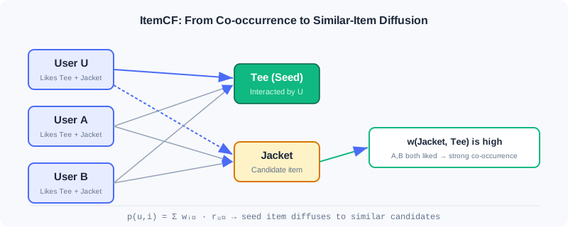
Whichever perspective you take, the core revolves around one concept — co-occurrence: two items interacted with by the same set of users, or two users interacting with the same set of items. The more frequent the co-occurrence, the higher the similarity. As we will see in the next three sections, all CF methods are just different answers to "how to define and exploit co-occurrence".
2.1.1 ItemCF: Item-Similarity-Based Collaborative Filtering
The core idea of ItemCF is that user interests are coherent: people who like an item tend to be interested in similar items. When recommending to a user, the system first identifies the items the user interacted with recently (seed items), then finds the most similar candidates for each seed, and finally aggregates the scores.
Computing Item Similarity
Most real-world scenarios have only implicit feedback (clicks, purchases), no ratings. ItemCF quantifies item similarity with cosine similarity:
where is the total number of users who interacted with item , and is the co-occurrence count of the two items (the number of users who interacted with both). The denominator normalizes the co-occurrence count, preventing popular items from dominating by sheer interaction volume — exactly the biggest trap of naive co-occurrence.
Recommending Candidate Items
Given the similarity matrix, the online flow has three steps: ① take a few hundred items the user recently interacted with as seeds; ② find the Top-10 similar items for each seed, quickly generating a large pool of candidates; ③ compute the user's interest score for candidate item :
is the set of items the user interacted with, and is the user's interest strength on item (set to 1, or weighted by interaction time/type). Finally, rank all candidates by score and take the Top-N.
🧠 Mental Model: A Borrower's Reading List
Think of items as "books" and users as "borrowers". ItemCF's logic: if Alice borrowed The Three-Body Problem and Ball Lightning, and Bob also borrowed The Three-Body Problem, then the system guesses Bob will probably like Ball Lightning too — because these two books are always borrowed by the same crowd. The point is not the content of the books, but "who reads them".
Computational Efficiency Optimizations
Brute-force computation of all item-pair similarities is , but the vast majority of item pairs share no common users, so their similarity is necessarily 0. A user–item inverted index speeds this up dramatically: maintain an interaction list per user, and when traversing, pair up items within each list, accumulate the co-occurrence matrix , then divide by the normalization terms. The optimized complexity is roughly ( is the total number of interactions, the average number of items per user), far below brute force in sparse settings.
Similarity for Rating Data (Pearson Correlation)
When the system has explicit ratings (e.g., 5 stars), the Pearson correlation coefficient is more robust than cosine, because centering removes differences in rating distributions across items:
Based on this, one can predict a user's rating for an unseen item:
In large-scale systems, for computational and sparsity reasons, most still use cosine similarity supplemented with weighted normalization.
Analysis: ItemCF can precompute the full item similarity matrix offline; online it only needs to fetch the Top-N similar items of the seed items, with very low latency and strong explainability. But it is powerless against item cold start (new items have no co-occurrence), and its similarity is fixed, hard to fuse with contextual features. It suits scenarios with stable item sets and dense interactions.
2.1.2 Swing: Similarity Optimization for Industrial Scenarios
ItemCF is naive and effective, but industrial deployment exposes clear problems: popular items dominate results due to high co-occurrence; noise such as random misclicks is treated equally. Swing offers an elegant answer — analyze substructures of the user–item bipartite graph to filter noise.
Its core insight: if multiple users bought the same pair of items despite sharing few other co-purchases, then the association between that pair is more trustworthy. In other words, the more "specific" the co-purchase behavior, the greater its contribution to similarity.
Computing Item Similarity
Let and be the sets of users who interacted with items and . For each pair of common users , if they share few other co-purchases (smaller ), then their joint choice of this item pair is more specific and should contribute a higher score:
is a smoothing coefficient preventing tiny denominators from causing numerical instability. To reduce the excessive influence of active users, a user weight is introduced:
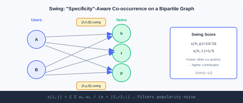
As shown, users A and B have 4 swing subgraphs , , , . If and A and B have 4 other shared behaviors, the user pair contributes ; h and p additionally share t and r, contributing two extra terms, so finally , higher than . Combinations with few but "exclusive" co-occurrences score higher — this is exactly how Swing filters popular-item noise.
Surprise: Complementary Item Recommendation
Swing scores already capture associations, but handling complementary items (buying a phone case after a phone) remains hard — complementary relations are directional and time-ordered. The Surprise algorithm measures complementary relevance at three levels: category, item, and cluster:
- Category level: compute conditional probabilities between categories with a user-category matrix, , and adaptively truncate the long tail using the maximum relative drop.
- Item level: consider purchase order and time interval — the closer in time, the stronger the complementarity:
- Cluster level: run label propagation on a graph of billions of items (edge weights are Swing scores) to cluster and alleviate sparsity, then combine linearly:
Analysis: Swing significantly improves robustness while preserving ItemCF's efficiency, making it an evergreen of industrial I2I retrieval; the cost is building and traversing the bipartite graph, with higher computation than naive ItemCF. Surprise goes further for complementary scenarios, but introduces multi-level hyperparameters and clustering steps, raising engineering complexity.
2.1.3 UserCF: User-Similarity-Based Collaborative Filtering
Mirror to ItemCF, UserCF assumes: users with similar historical behavior will have similar future preferences. It first finds the "neighbors" most similar to the target user, then predicts the target user's interests from the neighbors' behavior.
Computing User Similarity
Given users and with item sets and , three common measures:
- Jaccard coefficient (implicit feedback only):
- Cosine similarity (accounting for activity differences):
- Pearson correlation (with ratings; centering removes rating-habit differences):
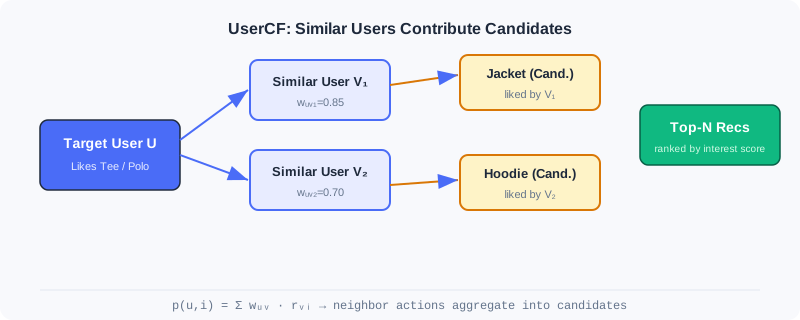
Recommending Candidate Items
Select the users with the highest similarity as the neighbor set . A simple weighted average predicts ratings:
The bias-aware version further removes personal habits:
At serving time, find the most similar users for the target user, collect their interacted items as candidates, compute interest scores , rank, and take the Top-N. The optimized complexity is roughly , far below .
Analysis: UserCF excels in scenarios where user interests converge, such as "trending news" or "breaking events", and naturally supports social recommendation through "discovering similar people". But when users vastly outnumber items, computation and storage costs are high, and user cold start is hard (new users have no behavior). In industry, ItemCF is more common, because its item set is stable and can be fully precomputed offline.
2.1.4 Matrix Factorization: From Similarity to Vector Representation
Both UserCF and ItemCF face a fundamental challenge: data sparsity. Real interaction matrices are extremely sparse, leaving too few common ratings to compute reliable similarities. Matrix factorization takes a different route — instead of explicitly computing similarities, it learns latent vector representations for users and items, letting distances in the vector space naturally reflect preferences. This marks CF's shift from statistical methods to machine learning methods.
The Dawn of the Latent Vector Era
Matrix factorization rests on two assumptions: the low-rank assumption — the seemingly complex rating matrix is actually governed by a few latent factors (such as "male-oriented vs. female-oriented", "serious vs. light"); and the latent vector assumption — every user/item can be represented by a vector encoding these factors.
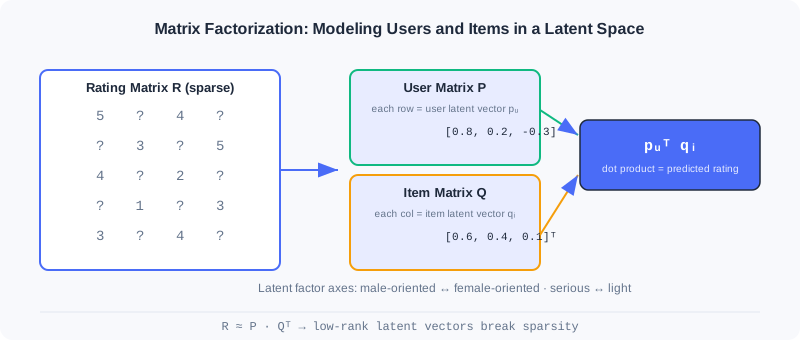
FunkSVD: The Basic Model
FunkSVD factorizes the rating matrix into a user feature matrix and an item feature matrix. User is represented by a -dimensional vector , item by , and the predicted rating is their inner product:
The optimization objective makes predictions approximate true ratings (over known ratings only):
Update with gradient descent, where the error is :
In practice, add L2 regularization against overfitting: .
🧠 Mental Model: Taste Axes
Plot every user and every movie on a 2D chart: the horizontal axis is "male-oriented ↔ female-oriented", the vertical axis "serious ↔ light". Users who like The Princess Diaries and the movie itself both land in the "female-oriented, light" corner, so the inner product is naturally large. Even if two users have never watched the same movie, as long as they are close on the latent factors, they can recommend for each other — this is the key to how vector representation overcomes sparsity.
BiasSVD: The Improved Model
The basic model ignores a fact: some people are naturally generous raters ("pushovers"), others strict; some movies universally rate high due to star casts. BiasSVD introduces bias terms:
is the global average rating, the user bias, the item bias. The optimization objective updates the biases as well:
Analysis: Matrix factorization handles sparse data naturally (two users can be linked through latent factors without any shared rating), and inner-product retrieval is efficient. But it remains a linear model, hard to fuse with side information or complex feature crossings. This leads directly to the two-tower and deep models of later chapters.
⚠️ Common Mistakes in 2.1
| # | Mistake | Example | Why It's Wrong | Fix |
|---|---|---|---|---|
| 1 | Using raw co-occurrence counts as similarity | Popular items appear "highly similar" to everything | No normalization in the denominator; popular items dominate by volume | Normalize with cosine similarity dividing by |
| 2 | Using ItemCF / UserCF interchangeably | Forcing UserCF in a user-cold-start scenario | New users have no history, so UserCF can't find neighbors | For user cold start use ItemCF; for item cold start use attribute/vector methods |
| 3 | Using Pearson as cosine | Forcing Pearson in an implicit-feedback setting | Without ratings there is no mean to center on | Use cosine for implicit feedback; Pearson only when ratings exist |
| 4 | Ignoring MF's sparsity precondition | Believing MF always computes accurate similarities | With extremely few interactions, latent vectors are poorly learned | For sparse data, combine side info (see EGES in Section 2.2) or two-tower models |
| 5 | Assuming CF can incorporate context | "Add time/location features into ItemCF" | Neighborhood methods have no feature-crossing channel | Representation learning (MF/two-tower) is needed to fuse features |
Chapter Summary
📌 Key Takeaways
| Concept | Key Points | Why It Matters |
|---|---|---|
| ItemCF | , expand candidates from seed items | A key industrial I2I retrieval channel, precomputable offline |
| Swing | Bipartite-graph specific co-occurrence + user weights | Filters popular-item noise, improves similarity robustness |
| UserCF | Aggregate neighbor behavior by user similarity | Great for trending/social scenarios, but user cold start is hard |
| Matrix Factorization | , low-rank latent vectors | Overcomes sparsity, pioneering vectorization |
| BiasSVD | Adds bias terms | Separates systematic biases, notably improving accuracy |
❓ FAQ
Q1: When should I use ItemCF vs. UserCF?
A: Use ItemCF when the item set is stable and you need to explain "why this similar item is recommended" (the industrial mainstream); use UserCF when user interests strongly converge (e.g., breaking news) or for social "similar people" recommendation. In user cold-start scenarios, ItemCF is more robust.
Q2: What exactly is the difference between cosine similarity and Pearson correlation?
A: Cosine only looks at the angle between interaction vectors and is affected by absolute item popularity; Pearson first centers (subtracts respective means), removing rating-habit differences between "pushovers vs. strict graders" and focusing on relative trends. Prefer Pearson with rating data; use cosine for implicit feedback.
Q3: Why does matrix factorization handle sparse data better than ItemCF?
A: ItemCF needs two items to share interacting users before similarity can be computed; matrix factorization, through a shared latent-factor space, lets two users with no common ratings recommend for each other via close latent vectors, generalizing to unseen combinations.
🔗 Connections to Later Chapters
- 2.2 (Vector Retrieval I2I) ports sequence modeling (Word2Vec) into similarity learning, and uses item attention to solve MF's difficulty in fusing side info.
- 2.3 (Two-Tower Model) upgrades MF's inner-product idea to deep-network encoding, enabling efficient U2I retrieval.
- 2.4 (Sequential Retrieval) further captures temporal interest dynamics ignored by ItemCF/MF.
- 3.x (Ranking) later applies complex deep models to finely rank the thousands of candidates retrieved in this chapter.
Practice Problems
Work through all problems in order — they get progressively harder. Each has a complete solution you can reveal after trying it yourself.
Problem 2.1.1 — Similarity Normalization 🟢 Easy
User A has interacted with 100 items, user B with 10 items, and they share 5 common items. Compute the Jaccard coefficient, and explain what would go wrong if you instead used "raw co-occurrence count = 5" as the similarity.
💡 Solution (click to reveal)
Approach: Jaccard divides the intersection by the union.
Key points:
- Using the raw co-occurrence count 5 as similarity, anyone sharing 5 items with A would be judged "equally similar", ignoring the fact that A is extremely active (100 items).
- Normalization (Jaccard/cosine) lets the "relative overlap ratio" rather than the "absolute co-occurrence count" determine similarity, preventing active users/popular items from dominating.
Problem 2.1.2 — ItemCF Scoring 🟢 Easy
User has interacted with items , with interest strengths and . Item has similarity with and with . Compute the user's interest score for candidate item .
💡 Solution (click to reveal)
Approach: Apply the ItemCF interest formula .
Key points:
- The score accumulates linearly with similarity and interest strength; more seeds and higher similarities yield higher candidate scores.
- This is exactly the core of ItemCF: "take seeds → expand by similarity → aggregate scores".
Problem 2.1.3 — The Specificity Intuition of Swing 🟡 Medium
Consider two item pairs and . Users A and B both interacted with both pairs, and A and B's other shared behavior counts are 4 (for h,p) and 2 (for h,t). Let . Suppose has only this single pair of common users, while additionally receives a contribution of the same structure from another common user pair C and D. Compare and , and explain what Swing is trying to filter.
💡 Solution (click to reveal)
Approach: Per the Swing formula, each common user pair contributes .
- : only the A, B pair, .
- : A, B contribute ; C, D (also ) contribute another ; total .
Wait — here is actually higher? Note: Swing's "specificity" means this user pair shares few other behaviors. If A and B overlap only on h and t (few other shared behaviors), while on h and p they also share more items (many shared behaviors = 4), then the h, p association is "not exclusive enough". In the problem, the shared behavior count of h,t (2) is smaller than that of h,p (4), so the per-pair contribution of h,t is larger — meaning the co-occurrence of h and t is more specific and more trustworthy.
Key points:
- Swing penalizes generic users who "buy everything together" via , and boosts "exclusive co-occurrences".
- What it filters is spurious strong associations caused by random misclicks or generic popular items.
Problem 2.1.4 — FunkSVD Gradient Update 🔴 Hard
Given a known rating , current , , , no regularization. Compute by hand and after one gradient descent step (keep 3 decimal places).
💡 Solution (click to reveal)
Approach: First compute the prediction and the error.
Update rules: , .
Key points:
- The error is positive (prediction too low), so parameters shift upward overall, increasing the inner product toward 4.
- Each dimension's update is proportional to "the counterpart vector's component", reflecting the symmetry of the inner product.
🏆 Challenge: Design a Retrieval Combination
A short-video platform adds tens of millions of items daily, with an enormous long tail. Write about 150 words explaining how you would combine this chapter's ItemCF, Swing, and matrix factorization as multi-channel retrieval (what each channel is responsible for, how they complement each other), and identify which channel should backstop long-tail new items and why.
💡 Hint
ItemCF/Swing handles "behavior-similarity expansion", with Swing suppressing popular-item noise, making it better at mining long-tail associations; matrix factorization handles "latent-vector generalization" to cover sparse users. New items have no co-occurrence, so the CF channels will inevitably miss them — the backstop should be a vector channel that can fuse side info (think EGES in 2.2) or a two-tower model. Note this chapter's MF itself also struggles with brand-new items and needs external attributes.
Vector Retrieval (I2I)
📝 Before You Continue: It is recommended that you first read ItemCF and matrix factorization in 2.1. This chapter is a natural extension of the "treat items as vectors" idea — the difference is that similarity is no longer derived from co-occurrence statistics, but determined by dense vectors learned through sequence modeling.
Collaborative filtering in 2.1 defines similarity by "who interacted with what together". But if an item has barely been interacted with (cold-start new product), co-occurrence statistics fail. More fundamentally: co-occurrence only tells you "related", without encoding items as semantic vectors, making it hard to further fuse attributes or perform nearest-neighbor search.
The protagonist of this chapter is the sequence modeling idea of Word2Vec. It rests on a simple yet profound assumption: words appearing in similar contexts have similar meanings. When we replace "sentence" with "a user's behavior sequence" and "word" with "item", the same machinery learns item representations where "semantically close means vectorially close", usable for I2I retrieval. From the most direct Item2Vec transfer, to attribute-fusing EGES, to Airbnb writing business objectives into the sequence — you will see how this line of work inches ever closer to industrial reality.
After reading this chapter, you will be able to:
- Explain the core formula of Word2Vec Skip-Gram, and why negative sampling is indispensable
- Describe how Item2Vec applies the "user behavior sequence = sentence" mapping to I2I vector retrieval
- Explain how EGES's item-specific attention solves cold start and sparsity
- Analyze how Airbnb's global context and same-market negative sampling bake "booking conversion" into training
- Complete 5 graded practice problems, consolidating sequence-modeling retrieval
2.2.0 From Words to Items: A Structural Analogy
Word2Vec's success rests on "co-occurrence reflects semantics". In natural language, a sentence consists of words whose co-occurrence reflects semantics; in recommendation, a user's interaction history can be viewed as a "sentence", with items as the "words". This is Item2Vec's entire starting point — structural isomorphism, ready for transfer.
| Text World | Recommendation World |
|---|---|
| Word | Item |
| Sentence | User interaction sequence |
| Word co-occurrence | Items interacted with by the same user |
In the next four sections, you will see how this seemingly naive mapping supports an entire family of I2I vector retrieval methods.
2.2.1 Word2Vec: The Theoretical Foundation of Sequence Modeling
📎 This section covers only the intuition of Skip-Gram and its transfer to recommendation. For the CBOW architecture, structural details of the center-word/context-word two-way weight matrices /, the exact form of negative sampling, and word-vector analogy properties, see Appendix: Word2Vec Deep Dive.
Word2Vec includes two architectures: Skip-Gram (predicting context from the center word) and CBOW (predicting the center word from context). Skip-Gram performs better in recommendation and is more widely adopted.
The Skip-Gram Model
Given the center word at position of a sequence, the model maximizes the occurrence probability of all context words within its window (size ):
is the vector of word , and is the vocabulary size. Softmax ensures probabilities sum to 1, and the inner product in the numerator measures the similarity between the center word and the context word.
🧠 Mental Model: The Guess-the-Neighbor Game
Imagine playing "I say a word, you guess what's likely next to it". Hearing "king", you'd probably guess "queen" or "castle". Skip-Gram makes the model play this game: it doesn't ask "do these two words co-occur", but "given the center word, what words are most likely around it" — through repeated guessing, the model is forced to place semantically similar words at nearby positions in the vector space.
Negative Sampling Optimization
Computing the Softmax denominator directly requires traversing the entire vocabulary, which is prohibitively expensive. Negative sampling turns the multi-class problem into multiple binary-class problems:
where and is the number of negative samples. The intuition: raise similarity for real word pairs, lower similarity for randomly sampled negative word pairs. This paradigm is exactly the technical cornerstone of subsequent recommender model training.
Analysis: Skip-Gram + negative sampling is efficient and scalable, the theoretical prototype for direct transfer to recommendation; but it works on "words", so user behavior sequences must be correctly mapped into training corpora before it applies to recommendation.
2.2.2 Item2Vec: The Most Direct Transfer
Item2Vec's core insight is exactly the "structural isomorphism" from the previous section: treat user interaction history as a "sentence" and items as "words".
Model Implementation
Item2Vec directly adopts Word2Vec's Skip-Gram, but simplifies sequence construction — each user's interaction history is treated as a set rather than a sequence, ignoring temporal weighting (the window still depends on positions after sorting by time; it just no longer assigns different weights to different positions). The objective function stays the same:
where is an item, is the window size, and takes the same Softmax form as Word2Vec. After training, each item gets a dense vector, enabling nearest-neighbor search for I2I retrieval.
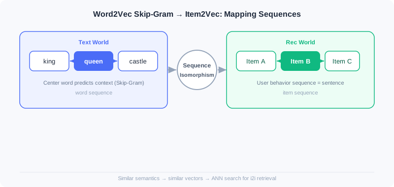
Analysis: Item2Vec is extremely easy to implement (a few gensim calls), validating the feasibility of sequence modeling in recommendation; but it treats history as an unordered set, losing temporal order, and is powerless against new-item cold start — no interactions, no vector. These two points are exactly EGES's motivation.
2.2.3 EGES: Enhancing Sequences with Attribute Information
Item2Vec treats interaction history as an unordered set and cannot handle cold start. EGES (Enhanced Graph Embedding with Side information) addresses both with two innovations: session-level graphs better reflect behavior patterns, and fusing side information solves sparsity and cold start.
Building the Item Relation Graph
EGES splits sessions by a "one-hour time window", building directed edges only between consecutive behaviors within the window, with edge weights as transition frequencies. Compared to treating the whole history as one sequence, this more accurately captures continuous interest transitions within specific periods. Weighted random walks on the graph generate training sequences, with transition probabilities determined by edge weights:
Fusing Side Information
Pure behavior sequences learn poorly for sparse items. GES first aggregates the item ID vector and attribute vectors with a simple average:
is the vector of the -th attribute, and is the item ID vector. But averaging assumes all attributes are equally important, which clearly doesn't hold (phones hinge on brand, daily necessities on price).
EGES's core innovation is item-specific attention — learning a set of weights per item to emphasize the more important attributes:
is a learnable weight. For cold-start new items with no behavior sequence and no trained , EGES degrades to mean pooling over attribute vectors, directly obtaining a meaningful representation so the item can be included in I2I retrieval.
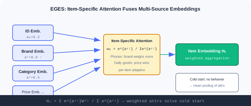
Training uses Word2Vec-style negative sampling, with the loss:
Analysis: EGES significantly alleviates sparsity and cold start with side information, outperforming traditional methods on billion-scale data; the cost is maintaining an attention parameter matrix of , raising engineering and storage costs. It represents the "balancing behavior and content" school of industrial I2I retrieval.
2.2.4 Airbnb: Baking Business Objectives into the Sequence
As a short-term rental platform, Airbnb has non-standard listings, bookings sparser than clicks, critical geography, and a stronger need to drive final booking conversion rather than mere similarity. It redefined the "sequence".
Business-Oriented Sequence Construction
- Session segmentation: a new session starts when the gap between user clicks exceeds 30 minutes, more accurately capturing coherent intent within a specific search context.
- Differentiated behavior weights: the final booking carries a much stronger preference signal than a plain click, and should receive higher weight in training.
The Global Context Mechanism
Traditional Skip-Gram only looks at local context within the sliding window. Airbnb forms positive pairs between the user's finally booked listing and every browsed listing in the sequence, no matter how far apart:
The first two terms are standard Skip-Gram (positive/negative samples); the third term is the innovation — the booked listing provides an extra learning signal for every listing in the sequence, letting the model capture "what kinds of listing combinations ultimately lead to a booking".
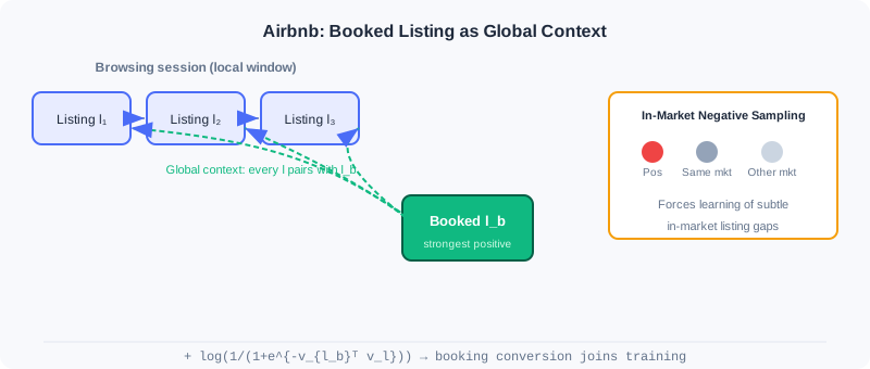
Market-Aware Negative Sampling
Users typically only book within the same market (city/region). If negative samples come from other regions, the model easily learns the easy "geographic location" feature while ignoring differences between the listings themselves. Airbnb draws some negative samples from the same market:
This forces the model to learn fine-grained differences between listings within the same region, improving discrimination.
Analysis: Airbnb writes "business conversion" and "geographic constraints" directly into the training objective, a model example of "business-objective-driven sequence construction"; but it is highly domain-customized (session thresholds and market partitions need business-specific tuning), less general than EGES.
⚠️ Common Mistakes in 2.2
| # | Mistake | Example | Why It's Wrong | Fix |
|---|---|---|---|---|
| 1 | Treating Item2Vec as an ordered sequence | Strictly sorting training data by timestamp | The Item2Vec paper treats history as an unordered set, losing temporal order | If order matters, use EGES/Airbnb/sequential retrieval (2.4) |
| 2 | Putting cold-start items directly into Item2Vec | New products have no vectors and can't be retrieved | No behavior means no co-occurrence, no learned vector | Use EGES's side-info mean pooling |
| 3 | Ignoring negative sampling | Computing full-vocabulary Softmax directly | Vocabulary/item corpus too large, computationally infeasible | Negative sampling approximation is mandatory |
| 4 | Applying Airbnb to non-geographic scenarios | Forcing market-based negative sampling on general e-commerce | Without geographic constraints it introduces noise instead | Business customization needs matching domain signals |
| 5 | Averaging attribute aggregation | Using simple averaging à la GES | Assumes all attributes are equally important, which doesn't hold | Use item-specific attention weighting |
Chapter Summary
📌 Key Takeaways
| Concept | Key Points | Why It Matters |
|---|---|---|
| Word2Vec Skip-Gram | + negative sampling | The theoretical cornerstone of sequence modeling, directly transferable to recommendation |
| Item2Vec | User sequence = sentence, item = word | Validates the feasibility of I2I vector retrieval |
| EGES | Item-specific attention | Fuses side info to solve cold start/sparsity |
| Airbnb | Global context + market-aware negative sampling | Writes booking conversion/geography into the objective |
❓ FAQ
Q1: What is the essential difference between Item2Vec and Word2Vec?
A: The architecture and objective function are identical; the only difference is the corpus — Item2Vec treats user interaction history as "sentences" and item IDs as "words", and by default treats history as an unordered set (losing temporal order). Word2Vec processes real text sequences.
Q2: Are EGES's attention weights the same thing as Transformer attention?
A: Not exactly. EGES's attention is a weighted aggregation across multiple attribute sources of the same item (static, per-item), used to obtain a single item vector; Transformer attention is dynamic interaction between tokens within a sequence. Both are called attention, but they operate at different levels.
Q3: Why does Airbnb add global context instead of relying only on the sliding window?
A: The sliding window only sees local neighbors, missing the strongest positive signal — the final booking (which may be far from the browsed listings). Global context pairs the booked listing with every browsed listing, reinforcing the learning of "what combination leads to conversion".
🔗 Connections to Later Chapters
- 2.3 (Two-Tower Model) uses deep networks to encode user/item vectors, upgrading I2I's "item vectors" to "user-item joint vectors" for U2I retrieval.
- 2.4 (Sequential Retrieval) explicitly models temporal order (LSTM/capsules), fixing Item2Vec's loss of order.
- 2.5 (Streaming Index) organizes massive vector indexes with clustering and streaming VQ, carrying forward the item vectors learned in this chapter.
Practice Problems
Work through all problems in order — they get progressively harder. Each has a complete solution you can reveal after trying it yourself.
Problem 2.2.1 — Negative Sampling Intuition 🟢 Easy
The Softmax denominator of Skip-Gram requires traversing the entire vocabulary . In recommendation, the item corpus can reach hundreds of millions. In one sentence, explain what problem negative sampling solves, and what form of task it converts the original objective into.
💡 Solution (click to reveal)
Approach: Recall that negative sampling turns "multi-class classification" into "multiple binary classifications".
Answer: Negative sampling converts "normalized Softmax over the full item corpus" into "binary classification on real pairs as positives + binary classification on a few randomly sampled negatives", avoiding a full-corpus traversal. That is, the multi-class problem becomes binary classifications (raise positive pairs, lower negative pairs).
Key points:
- The original objective contains , which is uncomputable.
- Negative sampling approximates with only sampled negatives, reducing complexity from to .
Problem 2.2.2 — The Item2Vec Mapping 🟢 Easy
Map the following text-world concepts to the recommendation world: (a) word (b) sentence (c) word co-occurrence. Also explain how Item2Vec is used for I2I retrieval after training.
💡 Solution (click to reveal)
Approach: Directly apply this chapter's mapping table.
- (a) word → item
- (b) sentence → user interaction sequence
- (c) word co-occurrence → items interacted with by the same user
Retrieval usage: After training, every item has a dense vector; take the nearest neighbors of a target item's vector (e.g., via ANN) to get the similar-item set as I2I candidates.
Key points:
- Structural isomorphism is Item2Vec's entire premise.
- Retrieval = nearest-neighbor search; no explicit co-occurrence matrix is needed.
Problem 2.2.3 — EGES Attention 🟡 Medium
EGES gives item a total of vectors ( attributes plus ID), with attention weights . Write the formula for the final vector , and explain: if a phone's "brand" weight is far higher than its "price" weight, what would mean pooling (GES) lose?
💡 Solution (click to reveal)
Approach: Write the weighted aggregation formula and compare with averaging.
Answer: Mean pooling (GES) weights all attributes equally: . If "brand" actually matters far more than "price" for phones, equal-weight averaging dilutes the key brand signal into a pile of weakly relevant attributes, yielding a more "mediocre" vector with reduced discrimination. EGES lets important attributes dominate via weighting, giving a sharper representation.
Key points:
- Attention is per-item; different items get different weight distributions.
- Equal-weight averaging assumes "attributes are equally important", which usually doesn't hold.
Problem 2.2.4 — Airbnb Global Context 🔴 Hard
In the third term of Airbnb's objective, , is the booked listing and is some browsed listing in the sequence. Explain: when is large (semantically close), how does this term's contribution to the loss change? How does this help the model learn "combinations that lead to bookings"?
💡 Solution (click to reveal)
Approach: Analyze the behavior of sigmoid and the log term.
: when is large, and (loss near 0, already learned); when is small/negative, and (strong penalty). So the third term maximizes , i.e., pulls the booked listing's and browsed listings' vectors together.
Answer: This term pulls every browsed listing's vector toward its booked listing. After training, browsed listings that frequently co-occur with a booked listing get pushed closer — the model thus learns the pattern "this kind of browsed combination ultimately leads to this kind of booking", and at retrieval time is more likely to surface listings that truly drive conversion.
Key points:
- Global context breaks the sliding window's local restriction.
- It is essentially giving the strongest positive signal — "booking" — a global weight.
🏆 Challenge: Design a Cold-Start I2I Solution
A platform adds 100,000 new products daily, 80% of which receive fewer than 5 interactions in their first week. Write about 150 words explaining how you would use this chapter's methods (any combination of Item2Vec / EGES / Airbnb) to build an I2I retrieval pipeline where new products can be retrieved despite minimal interactions, and identify what kind of data must be paired with it.
💡 Hint
New products have no behavior → Item2Vec is unusable; go the EGES route, using product attributes (category/brand/price/title vectors) with mean pooling to get cold-start vectors, then gradually refine them via random walks with "a few early interactions"; the platform must maintain a product side-info repository and a real-time behavior stream. See 2.5's streaming index for keeping vectors updated in real time.
Two-Tower Model (U2I)
📝 Before You Continue: Please first read matrix factorization in 2.1 and Item2Vec in 2.2. This chapter upgrades the "inner product" idea from item–item to user–item, encoding both sides with deep networks — the backbone of industrial U2I retrieval.
The item vectors you learned in the previous three sections (Item2Vec / EGES) perform I2I retrieval — first a seed item, then similar items. But online retrieval often starts not from an "item" but from a "user": given a user, pull out what they might like directly from a corpus of hundreds of millions of items. This requires a user representation and an item representation encoded separately in the same space, then retrieved by inner product — this is the two-tower model.
Its engineering charm lies in "divide and conquer": the item tower can be precomputed offline and stored in an approximate nearest-neighbor index (ANN), while the user tower computes in real time; online, only a single vector search is needed. From FM's mathematical prototype, to DSSM's deep encoding, to YouTubeDNN's "predict the next watch" — this chapter walks you through the two-tower evolution, with an interactive demo to build intuition for the retrieval process.
After reading this chapter, you will be able to:
- Derive the simplification of the FM second-order interaction term from to , and show how it reorganizes into a two-tower inner product
- Explain the role of DSSM's extreme multi-class training, vector normalization, and the temperature coefficient
- Describe YouTubeDNN's "asymmetric two-tower" and "temporal split" engineering tricks
- Understand the two-tower retrieval flow of "offline index building / online user query" through the interactive demo
- Complete 5 graded practice problems, consolidating two-tower representation and retrieval
2.3.0 Why Two Towers: From I2I to U2I
I2I retrieval depends on "the user has interacted with some item" as a seed. But in many scenarios, the user just registered, or we want to recommend before they take any action. U2I directly uses the user themselves (profile + behavior) as the query, retrieving candidates from the full corpus:
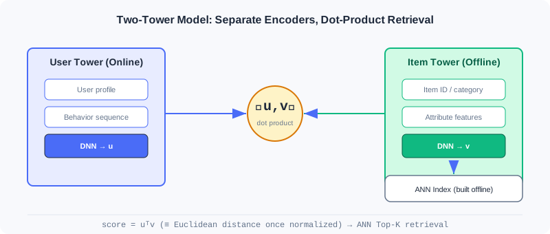
The two-tower's core convention: the two towers barely interact during training, meeting only at the final inner product. This buys a precious engineering property — item vectors can be computed offline once and indexed, user vectors computed online on the fly, with retrieval cost kept minimal.
2.3.1 FM (Factorization Machines): The Prototype of Two-Tower Models
FM was born before deep learning, yet anticipated the two-tower in spirit. It elegantly decomposes complex user–item interactions into the inner product of two low-dimensional vectors. The full expression:
Each feature corresponds to a -dimensional latent vector , with interactions modeled through the inner product .
Computational Complexity Simplification
The originally second-order term can be rewritten as:
Complexity drops from to , letting FM handle large-scale sparse data.
🧠 Mental Model: Latent Vectors as Building Blocks
Think of each feature as a block hiding a small pointer (its latent vector). Whether two features "get along" doesn't depend on the blocks themselves, only on whether their pointers point in the same direction (big inner product = compatible). FM's elegance: instead of exhaustively trying all pairs, it computes all pairings at once via "sum of squares minus square of sums".
Decomposition into a Two-Tower Structure
In retrieval scenarios, features fall into two groups: user side and item side . When recommending different items to the same user, interaction scores among user features are identical across all candidates and can be ignored during ranking. Keep only: intra-item interactions + user–item interactions. After rearrangement:
Look at the last term — it is exactly the inner product of two vectors and . Hence:
- User vector:
- Item vector:
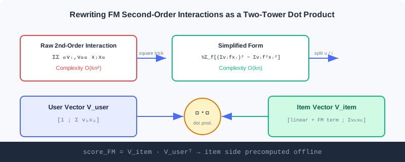
Analysis: FM uses linear algebra to turn feature crossings into a two-tower inner product, with item vectors precomputable offline — the theoretical prototype of the two-tower idea. But it is a linear model with limited expressiveness for complex nonlinear user–item relations — exactly why DSSM took over with deep networks.
2.3.2 DSSM: Deep Structured Semantic Model
DSSM replaces FM's linear transforms with deep neural networks, mapping users and items into a shared semantic space where similarity is measured by vector distance.
The Two-Tower Architecture in Recommendation
DSSM consists of two independent DNN towers: the user tower processes user features (behavior, demographics) and outputs a user embedding; the item tower processes item features (ID, category, attributes) and outputs an item embedding. The embedding dimensions of the two towers must match. Compared to FM's linear combination, DSSM lets each side perform complex nonlinear transforms within its own tower, with the two towers interacting only at the final inner product. Item vectors are precomputed offline, user vectors computed in real time, and retrieval is completed via ANN.
The Multi-Class Training Paradigm
DSSM treats retrieval as extreme multi-class classification: all items in the corpus are classes, and the goal is to maximize the predicted probability of the user's positive sample:
is the entire corpus. Since the corpus is huge, negative sampling approximates it in practice.
Key Details of Two-Tower Models
Vector normalization: L2-normalize both embeddings, . The raw dot product doesn't satisfy the triangle inequality, causing inconsistent "distances". After normalization, the dot product is equivalent to Euclidean distance:
The key is train/serve consistency — what training optimizes (normalized dot product) and what online ANN uses (Euclidean distance) are essentially equivalent, avoiding train-serving mismatch.
Temperature coefficient: divide the normalized inner product by :
amplifies similarity differences (more "confident"); smooths the distribution (more conservative). It essentially scales the logits, reshaping the Softmax output.
Analysis: DSSM's expressiveness comes from deep nonlinearity, and its engineering advantage from "offline item tower + online user tower". Normalization and temperature are the two must-tune knobs before launch — the former guarantees retrieval consistency, the latter controls retrieval "concentration". The cost is that the two-tower's "late interaction" loses some fine-grained feature-crossing signal.
2.3.3 YouTubeDNN: From Matching to Predicting the User's Next Action
YouTubeDNN is a milestone in two-tower evolution. It keeps the two-tower structure but introduces a key shift: defining retrieval as "predicting the user's next watched video", analogous to next-token prediction in NLP.
The Asymmetric Two-Tower Architecture
The user tower integrates multi-modal signals such as watch history, search history, and demographics; video IDs are embedded and aggregated by average pooling, with an Example Age feature introduced to model content freshness. The item tower is comparatively simple — essentially one huge embedding matrix, one learnable vector per video, avoiding complex item feature engineering. The objective is extreme multi-class classification:
Since the video corpus is huge, Sampled Softmax enables efficient training.
Key Engineering Tricks
- Asymmetric temporal split: instead of random validation, use "roll-over" — the prediction target only sees history before it, avoiding future leakage (matching real recommendation, where episodes are watched in order).
- Negative sampling strategy: importance sampling, computing only thousands of negatives each time, speeding training up by over 100x.
- Per-user sample balancing: generate a fixed number of training samples per user, preventing highly active users from dominating learning — critical for long-tail user performance.
Analysis: YouTubeDNN established the "scalable, production-ready" two-tower paradigm: train with a complex multi-class objective + rich user features; at serving time precompute item vectors, compute user vectors in real time, and pair with ANN retrieval. The asymmetric design keeps the item tower lean (easy offline indexing) while the user tower scales flexibly — a balance still widely borrowed today.
2.3.4 Interactive Demo: The Two-Tower Retrieval Process
The interactive demo below lets you feel the core flow of two-tower retrieval: the item tower encodes all items into a vector index offline; online, a user arrives, the user tower encodes their vector in real time, and nearest-neighbor search pulls the most similar Top-K candidates from the index. Click "Next" to observe each step.
Note the third step, "retrieve": it doesn't traverse the full corpus scoring every item, but uses ANN to locate directly in the neighbor space — this is the fundamental reason a two-tower can serve a corpus of hundreds of millions at millisecond latency. Normalization makes the inner product equivalent to Euclidean distance, and the temperature coefficient controls how concentrated retrieval is.
📊 Data Point: On the funrec benchmark, FM retrieval achieves hit_rate@10≈0.047, DSSM≈0.016, YouTubeDNN≈0.013. The numeric differences mainly come from dataset and feature configuration, not model quality — DSSM/YouTubeDNN usually win with richer features and larger scale.
⚠️ Common Mistakes in 2.3
| # | Mistake | Example | Why It's Wrong | Fix |
|---|---|---|---|---|
| 1 | Early interaction between towers | Concatenating user/item features early | Destroys the "items precomputable offline" property | Interaction happens only at the final inner product |
| 2 | Forgetting vector normalization | ANN retrieval on raw dot products | Dot product is not a metric; train-retrieve inconsistency | L2-normalize both sides |
| 3 | Careless temperature setting | Leaving τ=1 untuned | Retrieval concentration out of control, head over-clustering | Tune τ per business to shape the distribution |
| 4 | Treating FM as a deep model | "FM can fit any nonlinearity" | FM is linear with fixed crossing order | For nonlinearity, use DSSM |
| 5 | Random splits for YouTubeDNN | Validation set containing future behavior | Future leakage, inflated offline metrics | Use temporal roll-over splits |
Chapter Summary
📌 Key Takeaways
| Concept | Key Points | Why It Matters |
|---|---|---|
| FM, the two-tower prototype | Second-order interactions rearranged as | Theoretical starting point; items precomputable offline |
| DSSM | Deep two-tower + extreme multi-class + normalization/temperature | The industrial U2I backbone: expressive + efficient retrieval |
| YouTubeDNN | Predict next watch + asymmetric towers + temporal split | A scalable, production-ready paradigm |
| Train-retrieve consistency | Normalized dot product ≡ Euclidean distance | Avoids online/offline mismatch |
❓ FAQ
Q1: Why is the two-tower's "late interaction" actually an advantage?
A: Because item vectors can be fully computed offline and indexed; online, only the user vector plus one ANN search is needed. If towers interacted early (e.g., feature crossing), item vectors would depend on the specific user and become impossible to precompute, losing scalability.
Q2: What are the effects of increasing vs. decreasing the temperature τ?
A: τ<1 amplifies similarity differences — the model is more "confident" and retrieval more concentrated (prone to head clustering); τ>1 smooths the distribution, more conservative, with more dispersed candidates. It's the knob balancing precision and diversity.
Q3: Both FM and DSSM use inner products — what's the difference?
A: FM's vectors come from linear combinations + fixed latent vectors (a linear model); DSSM's vectors come from nonlinear transforms of deep networks (more expressive), and it explicitly handles normalization and sampled training.
🔗 Connections to Later Chapters
- 2.4 (Sequential Retrieval) upgrades user representation from "single vector" to "multiple vectors / long-short fusion", fixing the single two-tower vector's loss of temporal order.
- 2.5 (Streaming Index) takes the item vectors produced by two-tower models and organizes them into a streaming index that updates in real time.
- 3.x (Ranking) the ranking side can use more complex "early interaction" models (such as feature crossing), complementing the two-tower's late interaction.
Practice Problems
Work through all problems in order — they get progressively harder. Each has a complete solution you can reveal after trying it yourself.
Problem 2.3.1 — FM Complexity Simplification 🟢 Easy
FM's second-order interaction term in its original form requires pairing features two by two, with complexity . Write the simplified form, and explain why it only needs .
💡 Solution (click to reveal)
Approach: Recall the expansion of the squared term.
Answer: For each latent dimension , the right side only needs one pass over the features for the sum and the sum of squares, then subtraction: dimensions × features → instead of .
Key points:
- The key trick is turning "sum of pairwise products" into "square of the sum minus sum of the squares".
- This is exactly why FM scales to large sparse data.
Problem 2.3.2 — Two-Tower Inner Product Reorganization 🟢 Easy
In FM retrieval, intra-user-feature interactions are identical across candidates and can be ignored. The final score is written . Given user vector and item vector , compute the inner product (the matching score).
💡 Solution (click to reveal)
Approach: Multiply component-wise and sum.
Key points:
- The first term multiplies the constant 1 with the item vector's bias/linear part; the latter two terms are latent-vector interactions.
- The item vector is precomputed offline; online, only the user vector is computed plus one inner product.
Problem 2.3.3 — Normalization and Distance 🟡 Medium
Given unnormalized vectors , , . First use the raw dot product as "similarity" to judge who is closer to A (bigger dot product = closer). Then L2-normalize all three and judge with Euclidean distance . Explain why normalization is more reasonable.
💡 Solution (click to reveal)
Approach: Compute both ways.
Raw dot products: , . By "bigger = closer", C is closer. In this particular example that happens to agree with the geometry (, ), but the dot-product ranking is not reliable: it is distorted by vector magnitude — if C were replaced by a long vector like , which is not that close to A in angle, the dot product would still be large and the ranking would break. The unnormalized dot product is not a true distance metric.
After normalization: . Euclidean distances: , . Now C is closer (identical directions) and B farthest — matching intuition ( parallel, orthogonal).
Key points:
- The dot product is distorted by vector magnitude; it is not a true metric.
- After normalization, dot product ⇔ Euclidean distance; training (dot product) and ANN retrieval (Euclidean) are consistent.
Problem 2.3.4 — Temperature Effects 🔴 Hard
DSSM uses Sampled Softmax approximating . Given a user whose inner products with three items are . Compute the Softmax probabilities for and (formula ), and explain how τ affects retrieval concentration.
💡 Solution (click to reveal)
Approach: Substitute each case.
τ=0.5: , , sum=63.0 → .
τ=2.0: , , sum=5.367 → .
Answer: At τ=0.5, probability concentrates heavily on item 1 (0.866) — retrieval is very concentrated; at τ=2.0, the distribution flattens (0.506/0.307/0.186) — candidates disperse. Smaller τ is more "confident/concentrated"; larger τ more "conservative/dispersed".
Key points:
- τ scales the logits, reshaping the Softmax.
- Industry uses τ to balance "precise hits" against "diversity coverage".
🏆 Challenge: Design a Two-Tower Retrieval Pipeline
An e-commerce platform needs U2I retrieval with a 500-million-item corpus and peak 100K QPS. In about 150 words, explain: why two-tower over ItemCF; the division of labor between offline item-tower indexing cadence and real-time user-tower computation; and which link must use ANN, and why.
💡 Hint
Two-tower fits because "users without seed items can still be retrieved", item indexes can be built offline, and online only requires the user vector + ANN search — naturally suited to high QPS and large corpora; offline indexing can recompute item vectors into the ANN index in daily/hourly batches, while the user tower computes on request. ANN is indispensable — computing inner products against 500 million items one by one is infeasible; nearest-neighbor search is needed to return Top-K at millisecond latency. Temperature and normalization must be configured to keep retrieval consistent.
Sequential Retrieval
📝 Before You Continue: Please first read the two-tower model in 2.3. The MIND / SDM models in this chapter still do U2I retrieval, but user representation is upgraded from "single vector" to "multiple vectors / long-short fusion" — recovering the breadth of interests and temporal dynamics that two towers lose.
The two-tower model in 2.3 compresses a user into one vector. But this has two hidden dangers: user interests are diverse (you read programming books and buy running shoes), and they evolve dynamically (this session predicts your next need far better than last month's history). Summarizing "everything about a person" in one vector is like summarizing a person with a one-line label — not enough.
Sequential retrieval attacks exactly these two points. MIND uses multiple interest vectors (multi-interest capsules) to speak for different interests separately; SDM explicitly separates long- and short-term interests and fuses them dynamically with gating. With the interactive demo, you'll see clearly the advantage of "multi-vector retrieval" over single-vector retrieval.
After reading this chapter, you will be able to:
- Describe how MIND's dynamic routing (B2I) soft-clusters behaviors into multiple interest capsules
- Explain the roles of the squash function and label-aware attention in MIND
- Explain how SDM models the short term with LSTM + multi-head attention and the long term with feature-dimension attention, fusing them with gating
- Understand the "multiple interest vectors retrieve separately, then merge" flow through the interactive demo
- Complete 5 graded practice problems, consolidating sequential retrieval
2.4.0 Why a Single Vector Isn't Enough: Breadth and Temporality of Interests
Imagine your shopping history: programming books today, running shoes yesterday, coffee beans last week. With a single vector, these heterogeneous interests cancel each other out, averaging into a "neither-fish-nor-fowl" blob. Worse, the immediate intent in a short session (you just searched "running shoes") gets drowned out by long-term preferences.
The two themes of sequential retrieval: breadth (MIND: multiple vectors) and temporality (SDM: long-short separation). Let's break them down one by one.
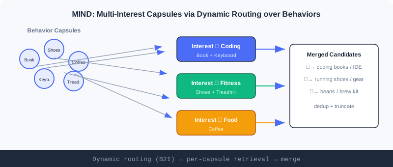
2.4.1 MIND: Capturing Diverse User Interests with Multiple Vectors
MIND (Multi-Interest Network with Dynamic Routing) borrows capsule networks' dynamic routing: soft-cluster historical behaviors by interest type, generating a dedicated interest vector per type. The core components are the multi-interest extraction layer and the label-aware attention layer.
Multi-Interest Extraction (B2I Dynamic Routing)
Historical behaviors are treated as "behavior capsules" and multiple interests as "interest capsules"; dynamic routing groups related behaviors onto the corresponding interest dimension. MIND makes three modifications to the original dynamic routing:
- Shared transformation matrix : all interest vectors live in the same representation space, easing subsequent similarity computation. Routing connection strength is ( behavior vector, interest capsule).
- Random initialization of routing coefficients : prevents all interest capsules from converging to the same state (similar to K-Means random centroid initialization).
- Adaptive interest count : users with few behaviors get fewer interest vectors, saving compute; active users get richer ones.
The Four Routing Iteration Steps
- Compute routing weights: Softmax over gives the soft assignment of behavior to interest :
- Aggregate behaviors: weight all behavior vectors (transformed by the shared matrix ) and sum, yielding a preliminary interest vector:
- Nonlinear squashing (squash): compress the magnitude to while keeping direction; magnitude is interpreted as the probability the interest exists, and direction encodes its attributes:
- Update routing coefficients: update by the consistency (dot product) between the new capsule and behaviors:
The four steps repeat about 3 times, outputting the interest capsule set .
🧠 Mental Model: Spokespersons for Each Interest
Think of MIND as assigning a "spokesperson" to each of a person's interests. Programming-related behaviors cluster to one spokesperson, sports to another, food to yet another. At retrieval time, each spokesperson goes to the item corpus to find candidates of "the kind they're responsible for", then all spokespersons' finds are merged — far better coverage than a single "averaged personality".
Label-Aware Attention
During training there is a "correct answer" (the item the user actually clicked next); use the target item's vector as the query to pick the most relevant of the multiple interests:
is the interest capsule matrix, the target item vector, and controls concentration: treats all interests equally; increasing sharpens the focus; degenerates into hard attention (pick only the most similar). Training uses Sampled Softmax to maximize similarity to the positive.
Analysis: MIND naturally expresses diverse interests with multiple vectors, with better retrieval coverage than a single vector; but there is no explicit temporal distinction among interests (capsules are parallel), and more heads bring redundant retrieval. This leads directly to SDM's explicit modeling of "temporality".
2.4.2 SDM: Fusing Long- and Short-Term Interests to Capture Dynamic Change
The core of SDM (Sequential Deep Matching) is to model the short-term immediate interest and the long-term stable preference separately, then fuse them intelligently.
Capturing Short-Term Interest (Three-Layer Structure)
- LSTM processes the current session sequence, learning temporal dependencies; its gating suppresses random misclicks:
- Multi-head self-attention captures multiple interests within the sequence:
- Personalized attention uses the user profile as the query to weight the multi-head output:
Capturing Long-Term Interest (Feature-Dimension Aggregation)
Long-term behaviors are split into subsets by feature: item ID, leaf category, first-level category, shop, brand . For each subset, attend with the user profile:
Concatenate the per-dimension representations and pass through a fully connected layer to get the long-term interest:
Fusing Long- and Short-Term Interest (Gating)
The gating network takes the user profile, short-term , and long-term , and outputs a 0~1 gating vector deciding per dimension the long/short contribution:
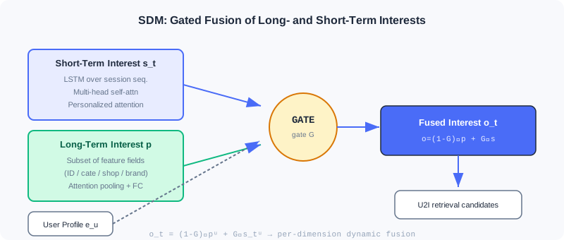
🧠 Mental Model: Long-Term Taste vs. Current Mood
Think of long-term interest as "your consistent taste" (loves sci-fi, prefers budget) and short-term interest as "your mood right now" (urgently buying running shoes). The gate is like a bartender: for different dimensions, pour more of the long term here, more of the short term there — neither a plain average nor one dominating the other, but per-dimension dynamic blending.
Analysis: SDM explicitly separates and fuses long/short term, modeling temporal dynamics more strongly than MIND; the cost is structural complexity (LSTM + multi-head + multi-feature-dimension attention + gating), with higher training and serving costs. Together with MIND it forms the two complementary routes of sequential retrieval: breadth vs. temporality.
2.4.3 Interactive Demo: Multi-Interest Vector Retrieval
The interactive demo below shows the MIND-style flow of "multiple interest vectors retrieve separately, then merge": the user's historical behaviors are clustered by dynamic routing into several interest capsules; each capsule retrieves its own Top-K from the item corpus; finally results are merged and deduplicated into retrieval candidates. Click "Next" to watch routing assign behaviors to different interests.
Note: a single-vector two-tower does one retrieval and easily averages away heterogeneous interests; multiple interest capsules each retrieve separately and merge, covering the "programming", "sports", and "food" threads simultaneously — exactly the key to MIND retrieving diverse long-tail content.
📊 Data Point: On the funrec benchmark, MIND achieves hit_rate@10≈0.0058 and SDM≈0.0555. SDM is significantly higher, partly because its explicit long-short fusion better matches the dataset's session pattern; both demonstrate the diversity gains of sequential retrieval over single vectors.
⚠️ Common Mistakes in 2.4
| # | Mistake | Example | Why It's Wrong | Fix |
|---|---|---|---|---|
| 1 | Treating MIND capsules as independent models | "Each capsule trains separately" | Routing is shared and iterative, trained end-to-end jointly | Understand the soft-clustering nature of dynamic routing |
| 2 | Ignoring the meaning of squash magnitude | Assuming direction is arbitrary | Magnitude = probability the interest exists | Constrain to [0,1) with squash |
| 3 | Naively concatenating long/short in SDM | "Concatenate and pass through a layer" | Loses information, hard to extract relevant parts | Use per-dimension dynamic gated fusion |
| 4 | Confusing MIND with multi-vector DSSM | "MIND is just several two-towers" | Routing soft-clusters, training uses label-aware attention | Distinguish "static multi-tower" from "dynamic routing" |
| 5 | Hard-coding the interest count K | Every user gets K=4 | Wastes compute on users with few behaviors | Use the adaptive |
Chapter Summary
📌 Key Takeaways
| Concept | Key Points | Why It Matters |
|---|---|---|
| MIND multi-interest | B2I dynamic routing + squash + label-aware | Multiple vectors express diverse interests, covering the long tail |
| SDM long-short fusion | LSTM+multi-head (short) / feature attention (long) / gating | Explicitly models interest temporal dynamics |
| Adaptive K | Allocates compute on demand | |
| Multi-vector retrieval | Each capsule retrieves separately, then merge | Complements single-vector two-tower |
❓ FAQ
Q1: What is the most fundamental difference between MIND and two-tower?
A: Two-tower gives each user one vector (single-vector retrieval); MIND gives each user multiple interest vectors (retrieve separately per vector, then merge). The former easily averages away heterogeneous interests; the latter covers multiple interest threads simultaneously.
Q2: Why does the squash function compress magnitude to [0,1)?
A: The capsule network convention is "magnitude = probability the interest exists, direction = the interest's attributes". Compressing to [0,1) lets the model express "how strong this interest is" via length, preventing unbounded vector growth and numerical instability.
Q3: Is SDM's gate the same thing as LSTM's gates?
A: Same spirit (both use sigmoid gating) but different roles: LSTM gates control "information flow within the sequence"; SDM's gate controls "the per-dimension fusion ratio between long- and short-term interests".
🔗 Connections to Later Chapters
- 2.5 (Streaming Index) solves "diverse/long-tail interests" from another angle — preserving full history with cluster statistics, complementary to multi-vector retrieval.
- 3.x (Ranking) sequence modeling (DIN/DIEN) on the ranking side further activates history with attention, echoing this chapter's retrieval.
- 2.3 (Two-Tower) is the "single-vector baseline" of sequential retrieval; understanding it is prerequisite to appreciating multi-vector gains.
Practice Problems
Work through all problems in order — they get progressively harder. Each has a complete solution you can reveal after trying it yourself.
Problem 2.4.1 — Adaptive Interest Count 🟢 Easy
A user has historical behaviors, with maximum interest count . Following MIND's adaptive formula , compute this user's actual interest vector count. Another user has only 3 behaviors — what is their ?
💡 Solution (click to reveal)
Approach: Substitute component by component.
User 1: , , → .
User 2: , ; implementations usually floor → effectively 1 (or 2, depending on floor/round). The formula's lower bound guarantees at least 1.
Key points:
- Active users cap at K; users with few behaviors automatically get fewer interests.
- Adaptivity avoids wasting multiple heads on sparse users.
Problem 2.4.2 — squash Magnitude 🟢 Easy
Given vector (magnitude 5). Use the squash formula to compute , give the magnitude and direction, and explain what the magnitude means.
💡 Solution (click to reveal)
Approach: Apply squash.
Magnitude ≈0.962, direction same as (i.e., ).
Key points:
- Magnitude is compressed to [0,1); here 0.962 means "this interest exists with high probability".
- Direction preserves the original attribute encoding; only the length is nonlinearly compressed.
Problem 2.4.3 — Gated Fusion 🟡 Medium
SDM gating: . Suppose a dimension has gate value , long-term value , and short-term value . Compute the fused result for this dimension and interpret it.
💡 Solution (click to reveal)
Approach: Substitute.
Answer: The fused dimension is 0.76, close to the short-term value 0.9. Since leans short-term, on this dimension "current mood" matters more than "consistent taste" (e.g., the dimension corresponds to immediate category intent).
Key points:
- Gating is per-dimension; different dimensions can lean long or short.
- The ratio is decided jointly by the user profile + long/short vectors, not globally fixed.
Problem 2.4.4 — Label-Aware Attention 🔴 Hard
MIND label-aware attention: . Suppose a user's three interest capsules have similarities with the target item . For and , compute the Softmax weights (formula ), and explain how focuses attention.
💡 Solution (click to reveal)
Approach: First compute .
p=1: , , sum=4.915 → .
p=10: ; after exponentiation the sum ≈ → .
Answer: At p=1, all three interests participate (weights 0.5/0.275/0.225); at p=10, attention is almost entirely on the most similar interest (0.99998). Larger p sharpens the focus; degenerates into hard selection.
Key points:
- pow amplifies differences, making the Softmax "sharper".
- A large p during training speeds convergence (explicitly choosing the most relevant interest).
🏆 Challenge: Designing a Combined Retrieval Setup
A content platform needs both "coverage of the user's diverse interests" and "tracking the current session intent". In about 150 words, explain how to combine MIND (multi-interest) and SDM (long-short term) as a two-channel sequential retrieval setup: what each channel is responsible for, how results are merged and deduplicated, and which channel better fits recommending "content the user has never shown interest in but wants right now".
💡 Hint
MIND's multi-interest capsules handle "breadth coverage" (programming/sports/food each retrieve separately); SDM's post-gating fused single vector handles "precision on current intent". Merge the two channels' Top-K, deduplicate by item, then truncate by similarity/diversity. SDM's short-term interest better fits "wants right now" immediate content, especially emerging in-session intent; MIND is better at awakening long-term diverse interests that were averaged away.
Streaming Index Retrieval
📝 Before You Continue: It is recommended that you first read the two-tower model in 2.3 and multi-interest in 2.4. This chapter steps outside the "compress history into vectors inside the model" paradigm, instead using the index structure itself to preserve full interests and update in real time.
The previous four sections all answer "how to encode users/items into better vectors". But there is an overlooked problem: models learning online tend to fit recent samples, gradually forgetting long-term, long-tail interests; meanwhile, traditional vector indexes require periodic rebuilds and cannot keep up with fast-moving content platforms.
Trinity and Streaming VQ in this chapter break through at the index level: the former uses cluster statistics to "explicitly preserve" full historical interests in histograms, never forgetting; the latter makes the vector quantization index update in real time as a stream, with no interrupted rebuilds. They represent the advancement of retrieval engineering from "compression inside the model" to "organization outside the index".
After reading this chapter, you will be able to:
- Explain Trinity's interest amnesia problem and its hierarchical clustering (VQ) solution
- Describe how the three histogram-based retrievers (diverse / long-tail / long-term) complement each other
- Explain how Streaming VQ replaces with to achieve a repairable, adaptive index
- Analyze the engineering value of index balance and the merge-sort serving strategy
- Complete 5 graded practice problems, consolidating streaming indexes
2.5.0 From Model Compression to Index Organization
The retrievers of previous chapters all compress user history into fixed-capacity vectors (single vector, multiple vectors, long-short fusion). Once capacity is fixed, old or rare interests can get "squeezed out" during training. Trinity proposes the opposite: don't compress inside the model — explicitly preserve in the index — aggregating historical behaviors into cluster histograms, where each cluster is an interest thread that is never forgotten.
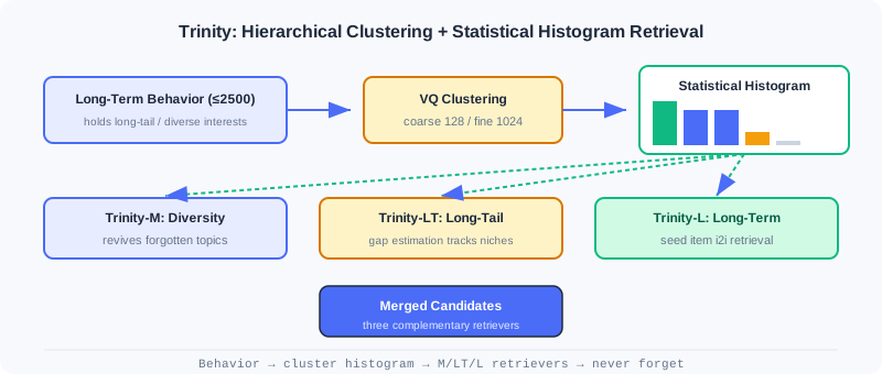
2.5.1 Trinity: Full-Interest Retrieval via Cluster Statistics
Trinity transfers "search-style interest modeling" to the retrieval stage, handling billions of candidates with a clustering-based statistical framework.
The Interest Amnesia Problem
Online learning frameworks tend to fit recent samples. When training samples for some interest topic become sparse, the model's memory of that topic fades — Trinity calls this Interest Amnesia. Long-term behavior reveals the full picture of diverse interests (short-term is dominated by popular content); the diverse interests truly worth attention are long-tail topics not yet sufficiently pushed; and judging whether a user is truly interested in the long tail requires going back to long-term behavior to confirm. The three are interdependent.
Building the Clustering System
The training stage uses vector quantization (VQ) to learn item cluster assignments. Maintain two levels of learnable cluster centroids: coarse primary clusters () and fine-grained secondary clusters (). Each item is assigned by nearest neighbor:
The training loss jointly optimizes user–item and user–cluster matching:
Cluster centroids are updated with exponential moving average (EMA) (weighted average of member item embeddings), smoothly adapting to distribution shifts. Because long-term behavior sequences are used simultaneously, recent and early items are treated equally — temporally unbiased, never over-favoring recent samples.
🧠 Mental Model: Ballot Boxes for Interests
Think of each cluster as a ballot box, and the user's historical behaviors as votes cast into the corresponding boxes. As long as the user once acted on that kind of content, the count in the box is non-zero — it can never be "forgotten". Trinity merely counts the votes per box and decides which interests to awaken by vote count. Compressing into a single model vector is like crumpling all the votes into one ball, drowning out the rare ones.
Histogram-Based Interest Retrieval
A behavior sequence of arbitrary length (up to 2500) is converted into a fixed-dimension statistical histogram: read each item's cluster ID, count behaviors per cluster, and obtain the primary cluster histogram and secondary . Sorted by descending count, the interest distribution is clear at a glance. For example, sorted counts correspond to clusters : cluster 10 is the dominant interest, 33/100 are diverse interests, 91/62 are exploratory interests.
Trinity accordingly designs three complementary retrievers:
- Diverse interest retrieval (Trinity-M): pick clusters with significant counts that may be ignored by the mainstream, at most one secondary cluster per primary cluster for dispersion — awakening "forgotten" topics.
- Long-tail interest retrieval (Trinity-LT): track cluster appearance intervals with streaming frequency estimation, ; large intervals = long-tail topics; boost pushes when the user has significant counts in these long-tail clusters.
- Long-term interest retrieval (Trinity-L): use a lightweight two-tower to pick seed items from long-term behavior, then perform I2I retrieval based on Trinity embedding similarity.
Comparison with Multi-Vector Methods
Multi-vector methods like MIND also capture diverse interests, but have flaws: different heads may redundantly retrieve popular content (efficiency drops as heads grow), semantics are unclear and hard to control, and extending to long-tail/long-term is hard. Trinity assigns items exclusively to clusters, so adding interest topics costs only linear overhead; each cluster has clear semantics (education/travel/tech), and the histogram never forgets — as long as relevant behavior exists in history, the corresponding count is non-zero.
Analysis: Trinity explicitly preserves full interests with statistical histograms, curing interest amnesia, with interpretable semantics and easy control; the cost is maintaining two-level cluster centroids with EMA updates, making index construction more complex than a single-vector two-tower. It represents the "organization outside the index" route.
2.5.2 Streaming VQ: A Streaming Index Updated in Real Time
Trinity solved interest amnesia, but the timeliness of the index structure remains: traditional vector indexes need periodic rebuilds, during which the mapping is frozen. On fast-paced platforms, new content pours in and trends churn — a frozen index can't keep up. Streaming VQ proposes a streaming-updated vector quantization index — items are assigned to clusters in real time, and centroids continuously adapt to the distribution.
The Core Mechanism of the Streaming Index
The training framework has two steps: the index step and the ranking step. The index step uses a two-tower to produce user/item embeddings, first optimized with an auxiliary task (in-batch contrastive learning) so that item vectors learn semantics independently of clustering:
Item embeddings are quantized to clusters by nearest neighbor:
The quantization centroids also participate in user–cluster matching optimization:
The item-to-cluster mapping is written to the parameter server in real time, centroids update via EMA, and the entire index updates live with training — no interrupted rebuilds.
Index Repairability
Streaming updates bring degradation risk (no periodic rebuild to "reset"). The original VQ-VAE constrains distance with , but in recommendation, data drift means cluster assignments should change dynamically — actually gets in the way. Streaming VQ replaces with : item embeddings update independently first, then adjusts centroids to the new distribution — the "items first" principle keeps clusters adapting continuously instead of locking items into outdated clusters.
Index Balance
Retrieval wants popular items spread evenly across clusters, so selecting a few clusters quickly narrows candidates. Streaming VQ promotes balance through multiple mechanisms:
- In 's softmax, popular items dominate samples; if they crowd into a few head clusters, centroids must represent many semantically diverse items with blurry representations and high loss; spreading across more clusters makes each centroid more consistent with lower loss — the optimization itself favors balance.
- EMA introduces popularity adjustment: ; niche items have larger gaps , gaining larger weights when , so centroids aren't dominated by popular items.
- Quantization introduces a perturbation ; clusters with sample counts below of the mean get , appearing "closer" and attracting items to join.
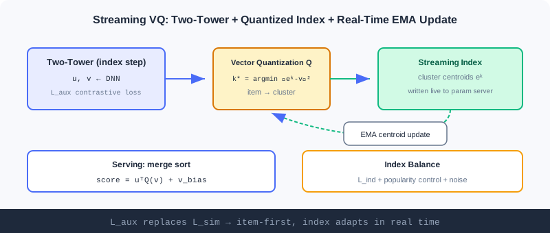
The Merge-Sort Serving Strategy
At serving time, the item embedding is decomposed into a personalization part and a popularity part:
is a global popularity bias, while carries the personalized matching. Clusters stay "grouped by semantics" without being skewed by popularity, and within each cluster provides the initial ranking. Use max-heap K-way merge sort: first rank at the cluster level by , then rank within each cluster by , guaranteeing every cluster a chance to contribute candidates.
Analysis: Streaming VQ keeps the index adapting to distributions in real time, repairable and balanced, with merge sort at serving time guaranteeing candidate diversity; the cost is real-time mapping writes to the parameter server + EMA maintenance, a heavier engineering pipeline than a static index. It complements Trinity: Trinity handles "interests never forgotten", Streaming VQ handles "the index never goes stale".
⚠️ Common Mistakes in 2.5
| # | Mistake | Example | Why It's Wrong | Fix |
|---|---|---|---|---|
| 1 | Assuming two-tower can remember the long tail | "A two-tower single vector covers all interests" | Fixed-capacity compression squeezes out the long tail | Explicitly preserve with histograms (Trinity) |
| 2 | Constraining VQ with L_sim | Adding a similarity loss to Streaming VQ | Blocks dynamic changes of cluster assignments | Replace L_sim with L_aux |
| 3 | Ignoring temporal unbiasedness | Training Trinity with only recent behavior | Reproduces interest amnesia | Train with long-term sequences simultaneously |
| 4 | Popular items piling into head clusters | Not intervening on index balance | Blurry centroid representations, poor matching | Rely on L_ind + popularity adjustment |
| 5 | Confusing Trinity with MIND | "Both are multi-interest, so they're the same" | The former is index statistics; the latter is model multi-vectors | Distinguish the index route from the model route |
Chapter Summary
📌 Key Takeaways
| Concept | Key Points | Why It Matters |
|---|---|---|
| Interest amnesia | Online learning forgets sparse long-tail interests | Motivates organization outside the index |
| Trinity histogram | Behaviors → cluster-count histogram → three retrievers | Explicitly preserves full interests, never forgets |
| Streaming VQ | L_aux replaces L_sim + real-time EMA updates | Index adapts in real time, repairable |
| Merge sort | score=uᵀQ(v)+v_bias, K-way merge | Guarantees candidate diversity and balance |
❓ FAQ
Q1: Trinity and MIND both address "diverse interests" — what is the fundamental difference?
A: MIND is inside the model with multiple interest vectors (online learning easily forgets sparse interests); Trinity is outside the index with statistical histograms explicitly preserving per-cluster counts — naturally never forgetting, with interpretable semantics and easy control.
Q2: Why does Streaming VQ use L_aux instead of L_sim?
A: L_sim locks items into old assignments "close to current centroids", blocking clusters from changing dynamically as data drifts; L_aux lets item vectors update independently first, then L_ind adjusts centroids — achieving "items-first" adaptation.
Q3: What does merge sort do at serving time?
A: It splits the score into "cluster-level personalization + within-cluster popularity", using K-way merge to give every cluster a chance to contribute candidates, preventing popular clusters from monopolizing and guaranteeing retrieval diversity.
🔗 Connections to Later Chapters
- 2.4 (Sequential Retrieval) is the "multi-vector inside the model" route, complementary to this chapter's "statistics outside the index"; the two can be combined.
- 2.3 (Two-Tower) the index step of Streaming VQ is exactly two-tower + quantization, carrying forward its vector outputs.
- Part 3 (Ranking) the candidates retrieved in this chapter proceed to the ranking stage for fine ranking.
Practice Problems
Work through all problems in order — they get progressively harder. Each has a complete solution you can reveal after trying it yourself.
Problem 2.5.1 — Reading the Histogram 🟢 Easy
Trinity converts a user's behavior sequence into a primary cluster histogram with descending counts , corresponding to cluster indices . Identify which clusters correspond to the dominant interest, diverse interests, and exploratory interests.
💡 Solution (click to reveal)
Approach: Stratify by count.
- Dominant interest: highest count (50) → cluster 10.
- Diverse interests: next highest, needing awakening (20,20) → clusters 33, 100.
- Exploratory interests: lower counts (4,2) → clusters 91, 62.
- The rest (21,5,83) have zero counts and can be ignored.
Key points:
- After descending sort, high counts = backbone, mid counts = diverse, low counts = exploratory.
- A non-zero count means that interest has not been forgotten.
Problem 2.5.2 — Quantization Assignment 🟢 Easy
Streaming VQ quantization formula: . Given item with vector and three cluster centroids , , . Find .
💡 Solution (click to reveal)
Approach: Compute squared distances to each centroid.
The minimum is 0 → .
Key points:
- Quantization = nearest-neighbor assignment; items go to the closest centroid.
- In streaming updates, this mapping is written to the parameter server in real time.
Problem 2.5.3 — The Interest Amnesia Intuition 🟡 Medium
A user's long-term behavior contains lots of "classical music", but the last 3 months include only popular "variety shows". An online-learning model gradually forgets the classical music interest. Explain: (a) why a two-tower single vector forgets; (b) why a Trinity histogram does not.
💡 Solution (click to reveal)
Approach: Compare how the two representations retain information.
(a) Two-tower single vector: The model fits recent samples online; gradients related to classical music are sparse, and its latent vector components get gradually overwritten/averaged by continuous gradients from recent popular samples; fixed capacity squeezes out rare interests — interest amnesia.
(b) Trinity histogram: The historical behavior counts for the classical-music clusters were long since written into the histogram, and training uses long-term sequences (temporally unbiased). As long as the behavior exists in history, the count is non-zero and will still be awakened at retrieval time — it doesn't depend on the model "remembering" it.
Key points:
- Single vector = information compressed into capacity; the rare gets overwritten.
- Histogram = information externalized as counts, permanently preserved.
Problem 2.5.4 — Merge-Sort Decomposition 🔴 Hard
Streaming VQ serving score: . Given the inner product of the user vector with an item's quantized vector as 0.6, and the item's popularity bias , compute the total score. Also explain: if two items have inner products 0.6 and 0.4 but values 0.1 and 0.5, how does merge sort use these two terms at the "cluster level" and "within cluster" respectively.
💡 Solution (click to reveal)
Approach: Substitute and explain the two-level ranking.
Total score .
Two items: A (inner product 0.6, bias 0.1) → 0.7; B (inner product 0.4, bias 0.5) → 0.9.
Answer: Merge sort first ranks at the cluster level by the personalization term (selecting clusters that best match the user's personalization), then ranks within each cluster by . This way clusters stay "grouped by semantics" (not skewed by popularity bias), while within clusters the global popularity provides the initial ranking. B, weak in personalization but high in popularity, ranks high within its cluster; A, strong in personalization, wins in another cluster-level ranking — every cluster gets a chance to contribute, guaranteeing diversity.
Key points:
- The decomposition decouples "semantic grouping" from "popularity".
- K-way merge guarantees candidates cover multiple clusters in balance.
🏆 Challenge: Combining Streaming Index Retrieval
A short-video platform's trends churn every minute, with an enormous long tail and drifting user interests. In about 150 words, explain how to combine Trinity (histogram multi-retriever) and Streaming VQ (real-time quantization index) to build retrieval: what each compensates for, how the index is maintained in real time, and why this beats a pure two-tower for this scenario.
💡 Hint
Trinity's three histogram retrievers explicitly preserve diverse/long-tail/long-term interests, curing two-tower forgetting; Streaming VQ uses L_aux+EMA to let the cluster index adapt to trend churn in real time, repairable and balanced. Item mappings are written to the parameter server in real time; two-tower-produced vectors enter the index via quantization. Better than a pure two-tower because: the long tail isn't drowned, trends don't go stale, and the index follows distribution drift without periodic rebuilds.
After the retrieval stage narrows hundreds of millions of items down to a few thousand candidates, ranking takes over the most critical job: precise scoring. Its goal is to compute, for every candidate, a predicted score that comes as close as possible to true user preference (typically click-through rate, conversion rate, and so on), then sort candidates into the best order. Ranking is the main battlefield for the generalization power of deep networks — the five chapters in this Part advance layer by layer along the thread of "how to make the model stronger, more flexible, and better aligned with the business."
This Part doesn't rush to pile up model names. Instead, it keeps asking one question: what shortcoming of the previous method does each new model solve? Only by reading with "motivation" in mind will you know which model to pick when facing a real business problem.
What This Part Covers
| Section | Topic | The Big Idea |
|---|---|---|
| 3.1 | Wide & Deep | Joint training of "linear memorization + deep generalization" sets the foundational ranking framework |
| 3.2 | Feature Crossing | From FM's second-order crossing, through DeepFM and xDeepFM, toward automatic high-order crossing |
| 3.3 | Sequence Modeling | DIN dynamically activates history per candidate; DIEN explicitly models the temporal evolution of interests |
| 3.4 | Multi-Objective Optimization | MMoE and PLE balance multiple objectives; ESMM's entire-space modeling resolves dependency bias |
| 3.5 | Multi-Scenario Modeling | Multi-tower and dynamic weights adapt to distribution shifts across scenarios, capturing both commonality and specificity |
What You'll Be Able to Do After This Part
- 🟢 Explain the division of labor between "memorization" and "generalization" in Wide & Deep, and why joint training matters
- 🟢 Distinguish the different motivations of FM's second-order crossing, xDeepFM's vector-wise high-order crossing, and AutoInt's adaptive crossing
- 🟡 Explain how DIN's local activation breaks through the "fixed-length user vector" bottleneck, and how DIEN further models interest evolution
- 🟡 Differentiate the essential difference and modeling strategies between multi-task (multiple objectives in one scenario) and multi-scenario (one objective across different scenarios)
- 🔴 Design appropriate multi-objective / multi-scenario architectures for businesses with dependency relationships (e.g., CTR × CVR) or seesaw conflicts
- 🟡 Locate each model in this Part on the chain of "solving the previous method's shortcomings"
Core Concepts
| Concept | Section | Relevance |
|---|---|---|
| Memorization vs generalization / joint training | 3.1 | The foundational design philosophy of deep ranking models |
| Factorized crossing (FM) parameter sharing | 3.2 | The core technique for easing sparsity and parameter explosion |
| Vector-wise / adaptive high-order crossing | 3.2 | Letting the model automatically capture feature interactions of arbitrary order |
| Local activation (attention) | 3.3 | The key to modeling user interests that shift with the candidate |
| Interest evolution / session modeling | 3.3 | Upgrading a static "bag of items" into a dynamic sequence |
| Negative transfer / seesaw / gating | 3.4 | Multi-objective conflicts and mitigation mechanisms |
| Entire-space modeling (sample selection bias) | 3.4 | Resolving training bias caused by CVR dependencies |
| Scenario-private/shared parameters / dynamic modulation | 3.5 | Balancing commonality and differences when transferring across scenarios |
Prerequisites
- You have read Part 1 (recommender system paradigms and the three-stage pipeline) and Part 2 (the retrieval algorithm family)
- You have read 1.3 Feature and Embedding Basics, understand sparse / dense features, bucketing, and embedding lookup; and know about MLPs, activation functions, and backpropagation
- You roughly know what business metrics like CTR (click-through rate) and CVR (conversion rate) mean
This Part is the natural downstream of retrieval in Part 2 — the candidates are ready, and now we learn how to score them "precisely."
Tips for This Part
- Read every model with its "motivation" in mind. When you meet a new model, first ask: what shortcoming of the previous method does it solve? Where do the structural differences lie?
- Formulas serve intuition. Understand "why it was designed this way" before looking at the math; formulas are just the precise notation for a design idea.
- Read the Advanced chapters comparatively. 3.2 and 3.3 are dense with structurally similar models — comparing them side by side in a table gets you twice the result with half the effort.
- Run the interactive demos. 3.2 and 3.3 each include an interactive HTML — use the "next step" button to get a hands-on feel for how high-order crossings and attention activation unfold.
Let's dive in! 🚀
Wide & Deep
📝 Before You Continue: Please read 1.3 Feature and Embedding Basics first and understand sparse / dense features and lookup vectors; also recommended: finish the retrieval chapters of Part 2 so you know the engineering position of "candidates ready, ranking must score precisely."
When you search for a product in an app and the system recommends it, a ranking model computed scores for hundreds or thousands of candidates in milliseconds behind the scenes. But before 2016, industrial ranking models faced an awkward trade-off: either memorize historical patterns or learn to generalize — having both was hard.
The Wide & Deep model (Google, 2016) offered a plain yet far-reaching answer: since both capabilities are needed, design two components and let them train jointly, each doing its own job. It remains the baseline model for countless recommendation businesses and the starting point of all subsequent deep ranking models. After reading this chapter, you will not only be able to explain its structure, but also understand "why the split was designed this way."
After reading this chapter, you will be able to:
- Distinguish memorization from generalization in one sentence each, with a recommendation scenario example for both
- Write out the linear formula of the Wide part and explain how cross-product features embody memorization
- Explain how the Deep part achieves generalization via Embedding + DNN, and how it fundamentally differs from Wide
- Recite the prediction formula of jointly trained Wide & Deep, and explain why Wide / Deep often use different optimizers
- Work through 4 leveled practice problems to consolidate the "memorization + generalization" design idea
3.1.0 A Seemingly Contradictory Pair of Goals: Memorization and Generalization
When building recommendation models, we often pursue two goals at once: memorization and generalization.
- Memorization means the model learns and remembers feature combinations that frequently co-occur in historical data, e.g., "users who bought A usually also buy B." It precisely captures explicit, high-frequency associations and gives users highly relevant recommendations — but is powerless when facing combinations it has never seen.
- Generalization means the model learns deep relationships between features and can handle combinations rarely seen in training, e.g., "item A and item C belong to the same category; users who like A may also like C." Even if the user has never interacted with C, the model can still make a reasonable recommendation.
💡 Key Insight: Memorization makes recommendations "precise"; generalization makes them "broad." Memorization alone traps users in a filter bubble and cannot handle new items; generalization alone loses those high-value historical strong rules. The essence of Wide & Deep is to give one model both capabilities.
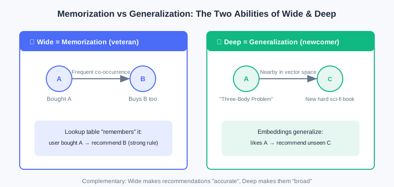
The memorization path on the left captures high-frequency strong rules like "people who buy A also buy B"; the generalization path on the right maps items into a vector space so the model can recommend similar items it has never seen (e.g., new books near The Three-Body Problem).
🧠 Mental Model: Veteran Employee vs Newcomer
Think of the Wide (memorization) part as an employee who has been at the company for twenty years: he remembers every historical "rule" (cross-product feature) — who always shows up with whom, he knows it cold. Think of the Deep (generalization) part as a systematically trained newcomer: he hasn't memorized all the rules, but knows how to reason by analogy and can handle combinations he has never seen. A good team needs both.
3.1.1 The Shortcut of Memorization: The Wide Part
The Wide part is essentially a generalized linear model (such as logistic regression). It is structurally simple, highly interpretable, and good at "memorizing" obvious association rules. Its mathematical form:
where is the prediction, the weights, the feature vector, and the bias.
The key of the Wide part is that the input contains not only raw features but also a large number of manually designed cross-product features. A cross-product feature combines multiple independent features into a new one to capture specific co-occurrence patterns. For example, in app store recommendation we can construct:
AND(installed_app=photo_editor, impression_app=filter_pack)
This stands for "the user has installed a photo editor AND is currently shown a filter pack recommendation." Through such cross features, the Wide part can directly and quickly learn strong associations like "photo editor users have a higher willingness to install filter packs" — a direct embodiment of memorization.
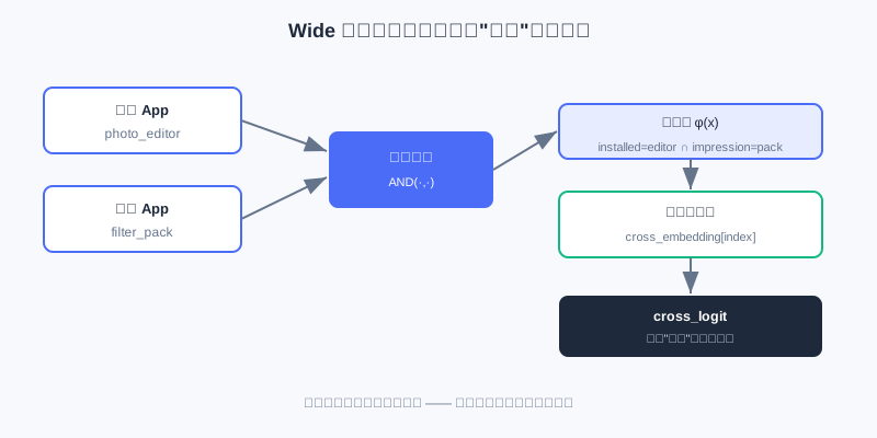
Raw features on the left (installed apps, impression apps) are combined by a cross function into a new feature, which then looks up an independent weight table, directly "remembering" the co-occurrence strength of that pair.
| Component | Role | Analogy |
|---|---|---|
| Raw features | Basic user/item attributes | Employee files |
| Cross features | Manually combined co-occurrence patterns | The "rules" in a veteran's head |
| Weights | Strong/weak memory for each combination | How much a rule is trusted |
💡 Key Insight: The essence of the Wide part's "memorization" is assigning an independent weight to every feature combination and directly remembering historical co-occurrences via lookup. The cost: these features must be hand-designed by experts, and they cannot generalize to unseen combinations.
3.1.2 Learning Complex Relations: The Deep Part
The Deep part is a standard feedforward neural network (DNN) responsible for the model's "generalization." Unlike Wide, which depends on manual feature engineering, the Deep part can learn high-order, nonlinear relationships between features automatically.
Its workflow has two steps. First, high-dimensional sparse categorical features (user ID, item ID) are mapped by an embedding layer to low-dimensional dense vectors — these vectors capture latent semantics. For example, the IDs of The Wandering Earth and The Three-Body Problem end up closer in the embedding space than The Wandering Earth and Boonie Bears. Then the embedding vectors are concatenated with other numerical features and fed forward through multiple layers:
where is the activation of layer , , are weights and biases, and is an activation function (such as ReLU). Layer-by-layer abstraction lets the DNN discover hidden complex patterns and make reasonable predictions for unseen feature combinations.
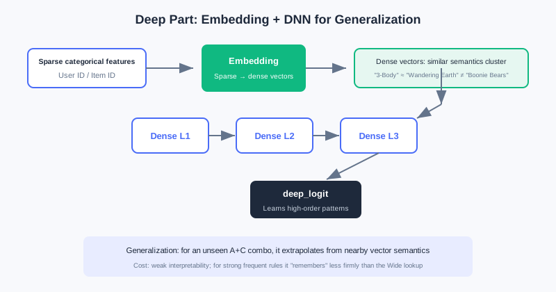
Sparse categorical features are first embedded into dense vectors (similar items get close in the vector space), then concatenated with numerical features and fed into a multi-layer DNN, automatically learning high-order nonlinear relationships.
Analysis: The Deep part excels at generalization and automatically learning feature interactions, but its interpretability is weak — the high-order combinations it learns are hard to read directly; and for very high-frequency strong rules it may not "stick" as firmly as Wide's explicit crossings. Complexity mainly comes from the deep MLP, with parameter count growing with layer width and depth; embedding lookup is cheap.
3.1.3 Combining the Two: Joint Training
Wide & Deep jointly trains both parts and combines their outputs for the final prediction:
Here is the Sigmoid function, is Wide's input (raw + cross features), and is the output vector of Deep's final layer. During backpropagation, gradients update all parameters of both Wide and Deep at once — this is "joint training," distinct from training separately and then ensembling.
An engineering detail worth noting: because the two parts handle parameters of different natures, they usually use different optimizers.
- The Wide part has sparse inputs, so the FTRL optimizer with L1 regularization is common. L1 produces sparse weights, effectively automatic feature selection, "remembering" only important rules.
- The Deep part has dense parameters, better suited to optimizers like AdaGrad / Adam.
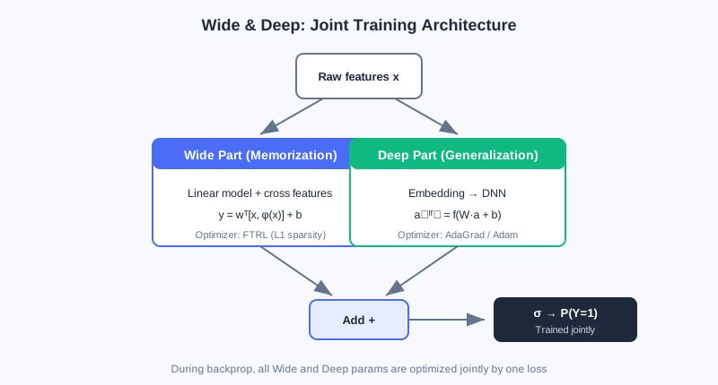
Wide (linear + cross features) and Deep (Embedding + DNN) share the input, each produces a logit, and the sum passes through Sigmoid to output the final click probability. The two parts are jointly optimized during training.
💡 Key Insight: The significance of Wide & Deep goes beyond a new architecture: it established a paradigm — how to combine "memorization" and "generalization" into one end-to-end model. It became the baseline of many ranking models and foreshadows later chapters (replacing manual crossings with FM, replacing fixed user vectors with attention).
⚠️ Common Mistakes in 3.1
| # | Mistake | Example | Why It's Wrong | Fix |
|---|---|---|---|---|
| 1 | Treating Wide as "another small DNN" | "Wide and Deep are both neural networks, just different depths" | Wide is linear + cross features, memorizing via lookup, not a nonlinear network | Remember: Wide = memorization (explicit rules), Deep = generalization (implicit learning) |
| 2 | Assuming cross features are discovered automatically | "Just throw raw features in" | Cross features require expert manual design; Wide will not combine them on its own | Understand Wide's limitation — exactly what FM/DeepFM later solve |
| 3 | Confusing joint training with ensembling | "Train Wide first, then Deep, then average" | Joint training is one loss, simultaneous updates of all parameters | Distinguish Joint Training (end-to-end) from Ensemble (separately trained) |
| 4 | Ignoring optimizer differences | "Just use the same Adam for both parts" | Sparse Wide suits FTRL (L1 sparsification); dense Deep suits AdaGrad | Pick optimizers by parameter nature: sparse → FTRL, dense → AdaGrad/Adam |
Chapter Summary
📌 Key Takeaways
| Concept | Key Points | Why It Matters |
|---|---|---|
| Memorization vs generalization | Wide memorizes high-frequency rules; Deep learns inductive generalization | Ranking models need both capabilities |
| Wide part | , memorizes via cross-feature lookup | Interpretable and precise on strong associations, but needs manual design and doesn't generalize |
| Deep part | Embedding + DNN automatically learns high-order nonlinearity | Strong generalization, no manual work, but weak interpretability |
| Joint training | End-to-end optimization of both parts; sets the ranking paradigm | |
| Optimizer split | Wide → FTRL (L1), Deep → AdaGrad/Adam | Matches sparse/dense parameter natures |
❓ FAQ
Q1: Since Deep is so strong, can we drop Wide and keep only Deep?
A: Pure Deep often "fails to stick" on high-frequency strong rules — it implicitly encodes rules into weights, unlike Wide's direct lookup. For high-frequency historical co-occurrences, explicit memorization is more stable and interpretable. Keeping Wide still has value.
Q2: Do cross features always have to be manually designed?
A: Wide's cross features are manual — that is exactly its shortcoming. FM / DeepFM in Section 3.2 were proposed precisely to learn feature crossings automatically and escape manual feature engineering.
Q3: Why is joint training better than "train Wide first, then Deep"?
A: Joint training uses one loss to update both parts simultaneously, so Wide and Deep calibrate each other during training; training separately and ensembling yields two independent models that cannot optimize end-to-end together.
🔗 Connections to Later Chapters
- 3.2 (Feature Crossing) replaces Wide's manual cross features with automatic FM, evolving into DeepFM with shared embeddings.
- 3.3 (Sequence Modeling) further breaks through the "fixed user vector," introducing attention to dynamically activate history.
- 3.4 (Multi-Objective) extends Wide & Deep's "two-tower / shared-bottom" idea into multi-task shared structures.
- The two-tower use of FM in Part 2 retrieval and FM for crossings in this chapter are two threads of the same technique.
Practice Problems
Work through all problems in order — they get progressively harder. Each has a complete solution you can reveal after trying it yourself.
Problem 3.1.1 — Distinguish Memorization from Generalization 🟢 Easy
For each recommendation behavior below, decide whether it mainly relies on "memorization" or "generalization," and explain why:
- (a) The system recommends the same brand of infant formula again to a user who "just bought infant formula yesterday" — because historically "people who bought formula re-purchase the same kind within 7 days" at a very high rate.
- (b) The system recommends to a fan of The Three-Body Problem a new book the user has never seen, tagged "hard sci-fi" like The Three-Body Problem.
💡 Solution (click to reveal)
Approach: Check whether the behavior is "remembering a high-frequency historical co-occurrence" (memorization) or "generalizing to an unseen combination" (generalization).
- (a) Memorization: it relies on the high-frequency historical rule "formula purchase → short-term re-purchase of the same kind," a direct application of explicit co-occurrence — exactly what the Wide part does.
- (b) Generalization: the user has never seen the new book; the model generalizes via "hard sci-fi" semantic similarity (proximity in embedding space), which is the Deep part's capability.
Key points:
- Memorization = direct reuse of high-frequency co-occurrence; generalization = inductive reasoning over unseen combinations.
- The two are complementary, and Wide & Deep has both.
Problem 3.1.2 — Complete a Cross Feature 🟢 Easy
A food delivery app wants its Wide part to memorize a strong rule: "users who browsed fast food on weekdays at lunch (12:00–14:00) are more likely to click afternoon-tea coupons." Write the corresponding cross feature in AND(...) form.
💡 Solution (click to reveal)
Approach: A cross feature combines multiple independent features into one new boolean feature capturing co-occurrence.
AND(time_slot=weekday_lunch, browse_cate=fast_food, impression=afternoon_tea_coupon)
Key points:
- Cross features are manually designed; experts must define which combinations are meaningful.
- This is exactly the Wide part's shortcoming, and the target FM later automates.
Problem 3.1.3 — The Joint Training Formula 🟡 Medium
The final prediction of Wide & Deep is . Answer:
- In the formula, where do and each come from?
- Why do Wide and Deep usually use different optimizers? Give one example of each.
💡 Solution (click to reveal)
Approach: Check against the joint training formula and optimizer split in 3.1.3.
- is the Wide part's input (raw features + cross features); is the output vector of the Deep part's last hidden layer.
- The two parts' parameters differ in nature: Wide's inputs are sparse (many 0/1 cross features), so FTRL fits better (L1 regularization yields sparse weights, automatic feature selection); Deep's parameters are dense, and AdaGrad / Adam converges more stably.
Key points:
- Joint training = one loss, simultaneous updates of both parts' parameters.
- The optimizer split by "sparse vs dense" is engineering experience, not a theoretical mandate.
Problem 3.1.4 — Memorization Failure on New Combinations 🔴 Hard
Wide & Deep outputs . Suppose a brand-new feature combination (a cross of two high-cardinality IDs) appears online that never occurred in the training set. Analyze: (1) what does the Wide part contribute for this combination; (2) can the Deep part give non-zero generalization; (3) to improve prediction quality on this combination, is it more worthwhile to modify Wide or Deep?
💡 Solution (click to reveal)
Approach: Examine each part's behavior on an "unseen combination."
- The Wide cross feature has no co-occurrence in training; its lookup weight (or randomly initialized and never updated), so Wide contributes almost no memorized signal for this combination — only first-order linear terms remain.
- In the Deep part, the embeddings of and are each well learned through co-occurrence with other features, so the DNN can give a non-zero generalized prediction via semantic proximity.
- The combination is "unseen," so Deep (generalization) should be the fallback; if it becomes frequent and important enough to deserve explicit memorization, add a Wide cross feature then. Modifying Wide does nothing for a new combination (no weight to look up), so Deep is the better deal.
Key points:
- Memorization failure = the lookup weight was never learned; generalization fallback = embedding semantics.
- This confirms "memorization + generalization are complementary" and exposes the cold-start weakness of Wide's manual crossings.
🏆 Challenge: Argue a Design Trade-off
Suppose you own ranking for an e-commerce app with tens of millions of daily active users. The business requires "capturing historical high-frequency hit combinations while giving newly listed long-tail items a chance." In at most 150 words, argue whether Wide & Deep fits, and state what would be lost if only half of it were kept.
💡 Hint
Wide captures high-frequency hits (memorization); Deep gives long-tail new items a chance via generalization. Keep only Wide and you're stuck in a filter bubble with poor cold start; keep only Deep and strong rules "won't stick" and interpretability weakens. Frame the argument around "neither capability can be missing."
Feature Crossing
📝 Before You Continue: Please read 3.1 Wide & Deep first. This chapter exists precisely to fix 3.1's shortcoming that "the Wide part needs manually designed cross features" — understanding Wide's limitation is what makes FM's motivation click.
The Wide part of 3.1 uses manual cross features to memorize strong rules, but hand-designing features is laborious and can never be exhaustive. A natural follow-up question arises: can the machine learn feature interactions by itself? That is exactly the problem feature crossing solves.
The most direct idea is to automatically capture interactions between all feature pairs — but recommender systems routinely have thousands of features; learning one parameter per pair would explode the parameter count; and the data is highly sparse, so most combinations have no training samples at all. In this chapter we start from FM's elegant factorization, walk all the way to automatic high-order crossing in xDeepFM and AutoInt, and include an interactive demo so you can "see" how high-order combinations are built step by step.
After reading this chapter, you will be able to:
- Explain how FM uses inner products of latent vectors to cut parameters down to and ease sparsity
- Distinguish the enhancements that AFM / NFM / PNN / FiBiNET each add on top of FM
- Explain how DeepFM replaces the manual Wide part with "shared Embedding" for an end-to-end model
- Compare the differing motivations of the three high-order crossings: DCN (element-wise) / xDeepFM (vector-wise) / AutoInt (adaptive)
- Work through 4 leveled practice problems, and use the interactive demo to understand how high-order combinations form
3.2.0 Motivation: From Manual to Automatic Crossing
The Wide part of Wide & Deep depends on experts hand-designing cross features, which has two pain points: (1) the combination space is too large for humans to enumerate; (2) newly appearing combinations have no ready-made feature. What we want is a mechanism that automatically learns interactions between arbitrary feature pairs without parameter explosion.
Recall FM from Part 2's retrieval: it factorizes users and items into vectors and uses inner products for efficient retrieval. At the ranking stage, FM shows a different face — its core idea of "learn one vector per feature, then capture interactions with vector inner products" solves exactly the pain points above. The same technique appears twice at different stages.
🧠 Mental Model: Give Every Feature a "Business Card"
Think of FM's latent vector as a "business card" handed to each feature, listing its interests. Want to know whether features A and B click? Instead of keeping a separate ledger for every A×B pair, just take the inner product of the two cards — high compatibility, large inner product. Even better: even if A and B have never appeared together in one sample, as long as each of their cards is well learned through other features, you can still infer the effect of A×B. That is the power of parameter sharing.
3.2.1 FM: Factorization Machines (Second-Order Crossing)
To capture feature interactions, a straightforward idea adds all second-order combination terms of the features to a linear model (a polynomial model):
It has two fatal flaws: (1) the parameter count is , unaffordable with many features; (2) in sparse data, most crossing terms never co-occur, so the corresponding weights cannot be learned.
FM's essence is parameter sharing: factorize each interaction weight into the inner product of two low-dimensional latent vectors, . Thus:
where are the -dimensional embeddings of features (). Instead of learning independent 's, each feature now needs only one -dimensional vector, bringing the total parameter count down to . More crucially: even if and never co-occur, as long as each co-occurs and learns well with other features (e.g., ), and are still valid, so the model can generalize to predict the effect of . Moreover, via an algebraic transformation, the FM second-order term's computation drops from to linear :
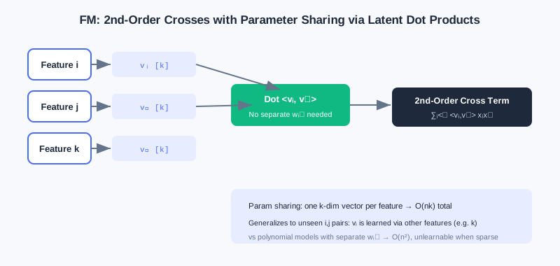
Each feature learns one -dimensional latent vector; the interaction of any two features is given by an inner product, with no per-pair weights — parameters drop from to .
Analysis: FM uses parameter sharing to solve both "parameter explosion" and "hard to learn under sparsity" at once, making it a widely used second-order crossing baseline in industry. Its limitation: it only models second-order pairwise interactions; higher-order combinations still rely on an upper DNN to learn implicitly, and the interaction form is a fixed "inner product" that cannot differentiate the importance of different crossings.
3.2.2 FM Family Enhancements: AFM / NFM / PNN / FiBiNET
FM treats all crossings "equally," but in practice different crossings matter to different degrees. Researchers have made various enhancements on top of it:
- AFM (Attention FM) introduces attention, assigning each pair a weight (Softmax normalized) so the model focuses on important interactions; the attention weights are visualizable and improve interpretability. Its interaction layer first computes the element-wise product , then does attention pooling: .
- NFM (Neural FM) feeds FM's second-order crossing result (in vector form) as "raw material" into a DNN to learn higher-order nonlinearity. The key is the Bi-Interaction pooling layer: , also optimizable to , then fed into an MLP. FM can be seen as the special case of NFM without hidden layers.
- PNN (Product-based NN) argues inner products / element-wise products each have limits, so its "product layer" uses inner products (IPNN) and outer products (OPNN) together to capture richer interactions, with matrix decomposition / superposition approximations reducing complexity from to .
- FiBiNET first learns feature importance (borrowing SENET from vision: Squeeze → Excitation → Re-weight), then uses bilinear interaction to break the symmetric-interaction constraint, combining "important features" with "flexible interactions."
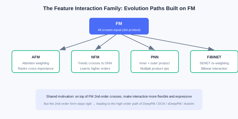
From "all crossings equally important" (FM) to "attention weighting" (AFM), "feeding a DNN" (NFM), "multiple product operations" (PNN), "re-weight first then bilinear" (FiBiNET) — the evolution always revolves around "more flexible, more expressive."
💡 Key Insight: These models all answer "how to do better on top of FM's second-order crossing" — some add attention (AFM), some attach deep networks (NFM), some change the product form (PNN), some select important features first (FiBiNET). But their second-order crossing form remains fairly fixed.
3.2.3 DeepFM: Unified Low-Order and High-Order Modeling
The Wide part of 3.1 needs heavy manual feature engineering. DeepFM simply replaces Wide with manual-free FM and lets FM and Deep share the same set of embeddings. Two benefits follow: (1) low-order and high-order interactions are learned together; (2) the shared embedding makes training more efficient.
DeepFM consists of two parallel components, FM and DNN, with shared inputs:
- The FM component captures first- + second-order crossings: .
- The Deep component concatenates all embeddings and feeds them to a DNN to learn high-order nonlinearity: , .
The two logits are summed and passed through Sigmoid: .
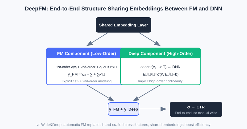
FM and DNN share one set of embeddings: FM learns low-order (first + second), DNN learns high-order, and their sum gives the final prediction — manual Wide features eliminated entirely.
Analysis: DeepFM's biggest improvement over Wide & Deep is replacing the manual Wide part with automatically learned FM, achieving a truly end-to-end model. Complexity mainly comes from the parallel FM + DNN, but the shared embedding avoids doubling parameters. Limitation: FM explicitly models only second order; higher orders still rely on the DNN implicitly, and the interaction form is fixed.
3.2.4 High-Order Crossing: DCN (Residual High-Order)
The FM family explicitly models second order; higher orders are mostly learned implicitly by the DNN, and we can't tell which order the DNN actually learned. DCN (Deep & Cross Network) replaces the Wide part with a Cross Network, where every layer crosses with the original input , thereby explicitly learning high-order interactions:
This is a residual structure: layer adds a "cross with the original input" term on top of the previous layer's output. The deeper the network, the higher the crossing order — layer 1 contains second order, layer 2 contains third order, and so on — while the parameter count grows only linearly with the input dimension. The Cross Network runs in parallel with the Deep Network, and their concatenated outputs go through logistic regression:
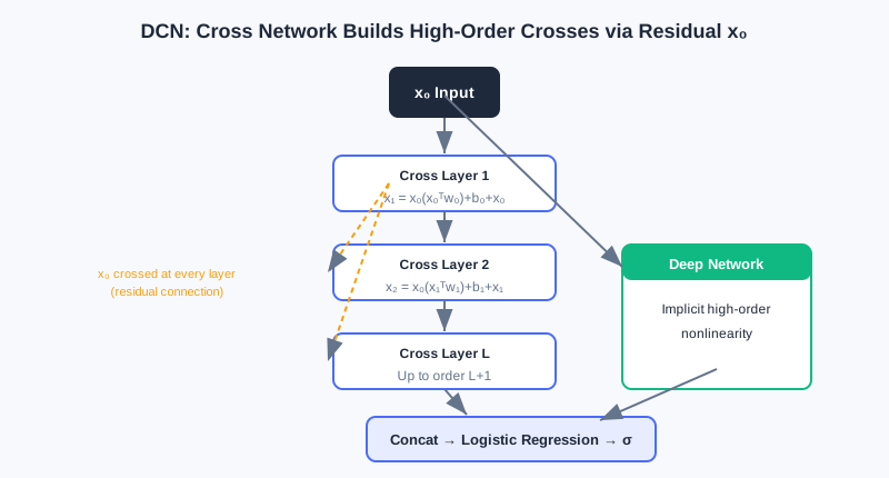
Each layer : the residual connection preserves the original information, continual crossing with raises the order with depth, and parameters grow only linearly.
Analysis: DCN learns arbitrarily high-order crossings explicitly and controllably, with efficient (linear-in-dimension) parameters. But it is an element-wise (bit-wise) crossing — every element of an embedding interacts separately, tearing the vector apart instead of treating the embedding as a whole feature. That is exactly what xDeepFM corrects.
3.2.5 xDeepFM: Vector-Wise CIN Interactions
DCN crosses at the element level; xDeepFM proposes the Compressed Interaction Network (CIN) and switches to vector-wise interactions, which better match intuition. xDeepFM has three components: linear + DNN (implicit high-order) + CIN (explicit high-order vector-wise), merged at the end.
The core of CIN: the layer- output is a weighted sum of all pairwise Hadamard products between the previous layer and the original input :
where is the vector-wise Hadamard product, preserving the -dimensional vector structure. Layer 's output contains all -order vector-wise interactions. The feature maps of each layer are concatenated after Sum Pooling, then merged with the linear and DNN outputs through Sigmoid:
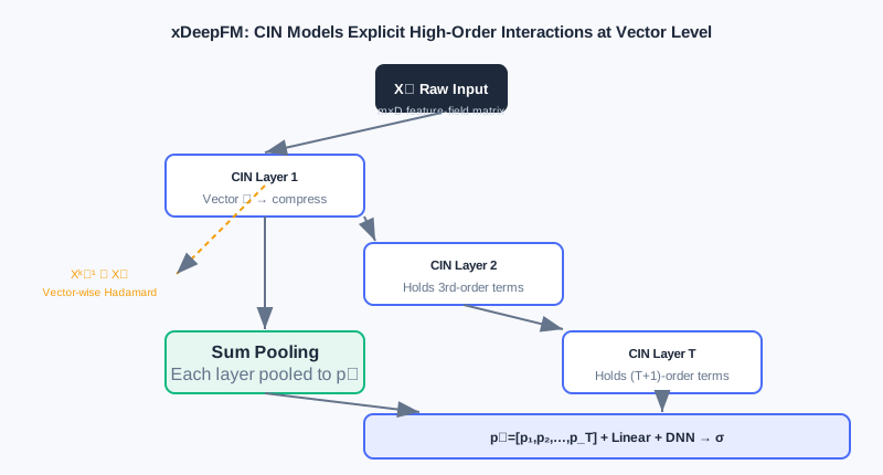
Each CIN layer takes vector-wise Hadamard products of "previous layer's feature maps × original input," then compresses them with weights into new feature maps; stacked layer by layer, this yields vector-wise crossings from second order up to T+1 order.
Analysis: xDeepFM combines "explicit vector-wise interactions" with "implicit element-wise interactions," gaining expressiveness and interpretable interactions (which layer corresponds to which order). The cost is the extra computation of the weighted vector sums in CIN, so the number of feature maps must be set carefully.
3.2.6 AutoInt: Self-Attention Adaptive Interactions
Each DCN layer crosses with in a fixed way, and xDeepFM's CIN also interacts in a fixed manner. AutoInt changes the approach: let the model decide which features interact and how strongly — using the Transformer's self-attention to adaptively learn interactions of arbitrary order.
For features , the relevance score of attention head :
The scores weight and sum the Values to obtain the new representation ; multi-head outputs are concatenated with residual connections added. Stacked layers: the first layer contains second order, the second contains third order, and so on — the interaction pattern is entirely determined dynamically by attention weights. Finally, all layers' representations are concatenated and fed to logistic regression.
💡 Key Insight: The motivational differences among the three high-order crossings are clear at a glance — DCN crosses in a fixed residual way (element-wise), xDeepFM crosses in a fixed CIN way (vector-wise), and AutoInt crosses adaptively with attention. The first two hard-code the interaction pattern; AutoInt leaves "who interacts with whom, how strongly" to the data, which is more flexible and interpretable (inspect the attention matrices).
3.2.7 Interactive Demo: How High-Order Crossings Form Layer by Layer
The interactive demo below gives a hands-on feel for how combinations "second order → third order → higher" are constructed from base features step by step. Click "Next" to observe which new crossing combinations each layer adds.
The demo uses 4 base features (e.g., gender, city, category, price tier) and shows layer by layer: layer 1 produces all second-order combinations, layer 2 crosses second-order ones with base features to get third order, and so on — exactly the intuition behind the explicit high-order crossings in DCN / CIN.
⚠️ Common Mistakes in 3.2
| # | Mistake | Example | Why It's Wrong | Fix |
|---|---|---|---|---|
| 1 | Thinking FM learns an independent weight per feature pair | "FM has crossing weights" | FM shares parameters via latent-vector inner products, only | Remember: ; parameters scale linearly in |
| 2 | Overlooking FM's significance for sparsity | "If features never co-occur, nothing can be learned" | Latent vectors are learned indirectly via co-occurrence with other features, enabling generalization | Parameter sharing is FM's core answer to sparsity |
| 3 | Treating DeepFM as identical to Wide & Deep | "DeepFM also needs manual cross features" | DeepFM replaces manual Wide with FM, end-to-end | Distinguish: Wide & Deep = manual crossing, DeepFM = automatic FM |
| 4 | Confusing DCN's and xDeepFM's crossing granularity | "Both are high-order crossing, no difference" | DCN is element-wise, xDeepFM is vector-wise | Check whether crossing happens on scalars or whole embedding vectors |
| 5 | Believing more high-order crossing is always better | "Stacking 10 Cross layers must be stronger" | Very high orders overfit, compute is expensive, and the business may not need it | Choose depth by data complexity and the validation set |
Chapter Summary
📌 Key Takeaways
| Concept | Key Points | Why It Matters |
|---|---|---|
| FM factorization | , parameters | Automatic second-order crossing solves parameter explosion + sparsity |
| FM family | AFM attention / NFM attaches DNN / PNN multiple products / FiBiNET re-weighting | Enhancements on top of second-order crossing |
| DeepFM shared Embedding | FM (low-order) + DNN (high-order) share input | End-to-end replacement of manual Wide |
| DCN residual high-order | (element-wise) | Explicit, controllable high-order crossing with linear parameters |
| xDeepFM CIN | Layer-by-layer compression of vector-wise Hadamard products | Vector-wise explicit high order, interpretable |
| AutoInt adaptive | Self-attention decides interactions and strength | Most flexible; interactions learned from data |
❓ FAQ
Q1: Why not just let a DNN learn high-order crossings — why FM/DCN?
A: A DNN can learn high orders implicitly, but we don't know which order or which combinations it learned, and sparse combinations are hard to guarantee. FM/DCN/xDeepFM make crossings explicit — controllable, interpretable, and friendlier to sparsity.
Q2: DCN or xDeepFM — which should I pick?
A: If feature interactions are better treated as "whole-vector" relations (e.g., semantic embeddings), xDeepFM's vector-wise form fits better; if simplicity and efficiency suffice and element-wise works, DCN is lighter. In practice, let the validation set and compute budget decide.
Q3: Can AutoInt's attention weights be used as feature importance?
A: Yes. The attention matrices directly show which feature pairs contribute to interactions — a major source of interpretability and one of AutoInt's advantages over DCN/xDeepFM.
🔗 Connections to Later Chapters
- 3.3 (Sequence Modeling) steps out of the "static feature bag" and adds the time dimension; DIN's attention shares its roots with the attention in AFM/AutoInt.
- The shared-bottom structures (Shared-Bottom/MMoE) of 3.4 (Multi-Objective) often use DeepFM-style models as the backbone.
- In Part 2 retrieval, FM is used for two-tower retrieval — two ends of the same technique as its ranking use in this chapter.
Practice Problems
Work through all problems in order — they get progressively harder. Each has a complete solution you can reveal after trying it yourself.
Problem 3.2.1 — FM Parameter Sharing 🟢 Easy
A recommendation scenario has features, and FM's latent vector dimension is . Answer:
- With the original polynomial model, roughly how many second-order crossing weights are there?
- With FM's latent-vector scheme, roughly how many parameters? How many orders of magnitude does that save?
💡 Solution (click to reveal)
Approach: Apply the order-of-magnitude formulas directly.
- The polynomial model's second-order term has about weights.
- FM needs only one -dimensional vector per feature: parameters.
Key points:
- From down to — roughly 2 orders of magnitude (a hundredfold).
- The gap widens as grows — the key to FM's industrial viability.
Problem 3.2.2 — Identify the Crossing Type 🟢 Easy
Match each description to the correct model among FM / DeepFM / DCN / xDeepFM / AutoInt:
- (a) Does residual crossing with the original input layer by layer, but tears apart every element of the embedding.
- (b) FM and DNN share one set of feature embeddings, learning low-order and high-order separately.
- (c) Uses multi-head self-attention to let the model decide which features should interact and how strongly.
- (d) Takes vector-wise Hadamard products of the previous layer's feature maps with the original input, then compresses.
💡 Solution (click to reveal)
Approach: Grasp each crossing's "granularity" and "whether it's adaptive."
- (a) DCN (element-wise / bit-wise residual crossing)
- (b) DeepFM (parallel FM + DNN with shared embeddings)
- (c) AutoInt (self-attention adaptive interaction)
- (d) xDeepFM (CIN vector-wise interaction)
Key points:
- Element-wise vs vector-wise: DCN vs xDeepFM.
- Adaptive vs fixed: AutoInt stands alone.
Problem 3.2.3 — Motivation Follow-up 🟡 Medium
Why can FM still give a reasonable prediction for the crossing when features and have never co-occurred in the training set? Explain using parameter sharing.
💡 Solution (click to reveal)
Approach: Explain from the perspective of "indirect learning" of latent vectors.
In FM the interaction weight is . Even if and never co-occur, can be learned well from 's co-occurrence with other features (e.g., ), and likewise from 's co-occurrence with . As long as these latent vectors are sufficiently well learned, their inner product can infer the tendency of — no direct samples of needed.
Key points:
- Parameter sharing lets "combinations never directly observed" still be estimated by generalization.
- This is FM's fundamental advantage over "independent weight per combination" in sparse settings.
Problem 3.2.4 — Derive FM's Linear Complexity 🔴 Hard
Starting from FM's second-order term , prove it equals , so the computation cost is . Also explain: when a feature , how are its interactions with all other features naturally ignored?
💡 Solution (click to reveal)
Approach: Expand the square and cancel terms.
. Rearranging gives . Both terms only require vector additions/squares over features followed by a sum — total instead of .
When , it contributes nothing to and , so every interaction term involving vanishes automatically — no explicit skipping needed; sparse features are ignored with zero wasted computation.
Key points:
- The algebraic transformation is what makes FM usable for high-dimensional sparse data.
- Interactions auto-zero when , a perfect fit for sparsity.
🏆 Challenge: Design a Crossing Scheme
A news app has 500 sparse features. It needs to capture second-order strong rules like "age × category," hopes the model automatically discovers patterns of third order and above, and requires an interpretable structure (being able to see which crossings matter). Pick a combination of 2 from FM / AFM / DCN / xDeepFM / AutoInt and justify your choice (within 150 words).
💡 Hint
Second-order + interpretable weights → AFM (attention visualization); high-order + interpretable order → xDeepFM (each CIN layer corresponds to a fixed order) or AutoInt (attention matrices). DCN is element-wise and can't directly show crossing importance, so you can skip it. A combination like "AFM + xDeepFM" covers interpretable low-order and interpretable vector-wise high-order.
Sequence Modeling
📝 Before You Continue: Recommended: finish 3.2 Feature Crossing first. Feature crossing treats user history as a "static feature bag"; this chapter introduces the time dimension — understanding this shift of perspective is the key to reading this chapter.
The various crossing models of 3.2 all aim to mine value from a static feature set. But they share a limitation: user history is treated as an unordered "bag of items." Yet user interests are not static — they have clear temporal structure and dynamic evolution.
Consider this difference: a user who browses "mouse" then "monitor" has a completely different purchase intent from one who browses "novel" then "monitor" — the former may be a digital enthusiast assembling a PC, the latter maybe just browsing casually. Traditional crossing models cannot capture intent encoded in order. In this chapter we upgrade user history from a "static bag" to a "dynamic sequence," and see how three representative industrial models — DIN / DIEN / DSIN — tame time.
After reading this chapter, you will be able to:
- Explain how DIN's local activation breaks through the "fixed-length user vector" bottleneck, and why its attention weights are not Softmax-normalized
- Explain how DIEN uses an auxiliary loss + AUGRU to explicitly model the temporal evolution of interests
- Describe how DSIN uses the "session" as its basic unit for hierarchical modeling (intra-session self-attention, inter-session Bi-LSTM)
- Use the interactive demo to observe how DIN dynamically activates different historical behaviors depending on the candidate ad
- Work through 4 leveled practice problems to consolidate the three pillars of sequence modeling: "dynamic / sequential / focused"
3.3.0 Motivation: From Static Feature Bag to Dynamic Sequence
On large e-commerce platforms, user interests are diverse: the same user may follow digital gadgets, watch sports content, and buy daily necessities. The traditional Embedding & MLP paradigm pools all of a user's historical behavior embeddings into one fixed-length vector to represent the user — and there's the problem: whether you recommend "running shoes" or "phones," the same vector represents them. Trying to cram all interests in "equally" is both difficult and insufficiently focused for the specific task.
💡 Key Insight: A user's concrete click is usually activated by only a fraction of their historical interests. When recommending a "mechanical keyboard" to a digital enthusiast, what really matters is their recent "gaming mouse" and "graphics card" behavior — not the running shoes they bought last month. Interest representations should change dynamically with the candidate.
🧠 Mental Model: Not a Resume, but a Spotlight
Think of the traditional "fixed user vector" as a static resume — all experience squeezed onto one page, identical for every reader. Think of DIN's "local activation" as a spotlight: when a candidate ad arrives, the light falls only on the few relevant segments of history while the rest dims. The candidate hasn't changed, but "how they appear under the light" changes with the interviewer (the candidate).
3.3.1 DIN: Attention via Local Activation
The core of the Deep Interest Network (DIN) is local activation: the user interest representation should not be fixed but should change dynamically with the candidate ad . To this end DIN introduces a local activation unit (attention) that computes a "weighted sum" over the embeddings of user 's historical behaviors:
where is the historical behavior embedding, is the candidate ad embedding, and the activation unit is typically a small feedforward network that takes and outputs weight . The more relevant a behavior is to the ad, the larger its weight, and the more it dominates the final interest vector.
A key detail: DIN's attention weights are not Softmax-normalized, i.e., is not necessarily 1. This preserves the absolute strength of interest — if most of the user's history is highly relevant to an ad, the weighted-sum vector has a large norm; otherwise, a small one. The model thus senses both the "direction" and the "strength" of interest.
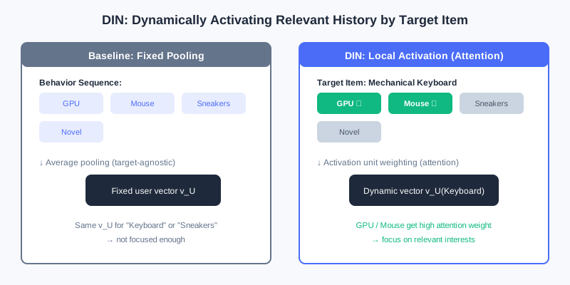
Left: the baseline model pools all history into a fixed vector (candidate-independent). Right: DIN uses an activation unit to compute attention per candidate; relevant history (graphics card, mouse) is highlighted and up-weighted while irrelevant history (running shoes) is down-weighted, yielding an interest vector that varies with the candidate.
Analysis: DIN breaks the fixed-vector bottleneck with lightweight attention, significantly improving expressiveness under diverse interests at small computational cost (just one added activation unit). Limitation: it still treats history as an unordered set, ignoring temporal dependencies between behaviors — interests evolve rather than stand still. Complexity mainly lies in the attention-scoring feedforward network, growing linearly with sequence length.
3.3.2 DIEN: Modeling Interest Evolution
DIN captures "diversity + local activation" but treats history as an unordered set, ignoring temporal dependencies. The Deep Interest Evolution Network (DIEN) asks: knowing what a user liked in the past is not enough — you must understand how interests change to predict the next step better. DIEN realizes this with a two-stage structure.
Stage one: the Interest Extractor Layer. A GRU processes the behavior embedding sequence over time. But can the GRU hidden state really represent "interest"? DIEN adds an auxiliary loss: the hidden state at time must predict the true next behavior (positive sample) against negatively sampled behaviors (negative samples):
It is added to the final CTR loss: . This extra supervision forces the GRU to learn more meaningful interest representations.
Stage two: the Interest Evolving Layer. With the interest state sequence in hand, a GRU with attention-based update gates (AUGRU) models the evolution. The attention score is determined by the interest state at time and the candidate ad : , which then scales the GRU update gate . Interest relevant to the candidate passes through smoothly, while irrelevant "interest drift" is suppressed.
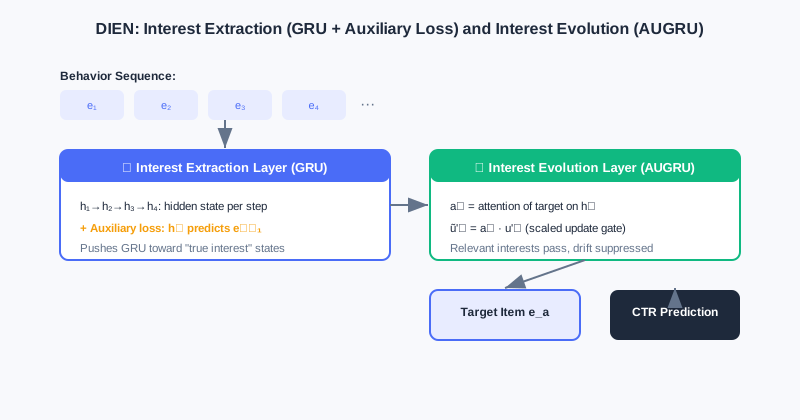
The interest extractor layer uses a GRU with the "predict the next behavior" auxiliary loss to learn true interest states; the interest evolving layer uses AUGRU (attention-scaled update gates) to let interest paths relevant to the candidate pass through while suppressing interest drift.
Analysis: DIEN explicitly models the temporal evolution of interests, matching the fact that "interests change" better than DIN, and performs better in scenarios with long sequences and obvious interest drift. The cost is a more complex structure — GRU + auxiliary loss + AUGRU bring higher training and inference costs — and the GRU's sequential computation is hard to parallelize.
3.3.3 DSIN: From Behavior Sequence to Session Sequence
From DIN to DIEN, interest understanding moved from "static relevance" to "dynamic evolution," but both treat behaviors as one continuous sequence. In reality user behavior is often interrupted: intent is concentrated within a session, while interests may shift dramatically between sessions. DSIN (Deep Session Interest Network) takes the "session" as its basic unit and models hierarchically.
DSIN has four layers:
- Session Division Layer: splits the long sequence into multiple short session sequences by time gaps (e.g., >30 minutes).
- Session Interest Extracting Layer: applies self-attention (Transformer-style) within each session to capture intra-session relations and aggregates into a session interest vector .
- Session Interest Interacting Layer: applies Bi-LSTM to the session sequence to capture evolution across sessions.
- Session Interest Activating Layer: weighted-sums session interests with attention based on the candidate ad (in the same lineage as DIN):
DSIN splits the long sequence into sessions: self-attention aggregates within each session (homogeneous), Bi-LSTM transfers across sessions (heterogeneous), and finally attention activates relevant sessions per candidate — a fine-grained depiction of "intra-session aggregation + inter-session transfer."
💡 Key Insight: The three sequence models embody three progressive ideas — dynamism (DIN: interest shifts with the task), sequentiality (DIEN: exploits temporal order and evolution), and focus (DSIN: hierarchical by session, activated by candidate). Together they upgrade the "static bag of items" into a "dynamic sequence that tasks can focus on."
3.3.4 Interactive Demo: DIN Attention Activation
The interactive demo below lets you feel DIN's core: given the same user (fixed historical behaviors), switching to a different candidate ad makes the highlighted, activated history completely different. Click "Next" to switch candidates and watch the spotlight move across different histories.
In the demo, the user's history includes "graphics card, mouse, running shoes, novel," and more. When the candidate is "mechanical keyboard," graphics card / mouse are activated; switch the candidate to "running socks" and the spotlight turns to running shoes — an intuitive display of "local activation."
⚠️ Common Mistakes in 3.3
| # | Mistake | Example | Why It's Wrong | Fix |
|---|---|---|---|---|
| 1 | Thinking DIN uses a fixed user vector | "DIN pools history into one vector" | DIN uses attention to dynamically generate a vector that changes with the candidate | Distinguish baseline pooling (fixed) vs local activation (dynamic) |
| 2 | Adding Softmax to DIN's attention | "Weights must sum to 1 to be proper" | DIN deliberately does not normalize to preserve interest strength | Understand: preserving the norm = preserving strength information |
| 3 | Assuming DIEN is just a GRU | "DIEN = two stacked GRU layers" | The crucial auxiliary loss and AUGRU are also there | Both stages are indispensable: extraction + evolution |
| 4 | Treating DSIN as a long-sequence RNN | "DSIN just runs one RNN over the whole sequence" | DSIN first splits by session, then models hierarchically (self-attention + Bi-LSTM) | The session is the basic unit; model hierarchically |
Chapter Summary
📌 Key Takeaways
| Concept | Key Points | Why It Matters |
|---|---|---|
| DIN local activation | , weights not Softmax-normalized | Interest varies with the candidate, breaking the fixed-vector bottleneck |
| DIEN evolution | GRU + auxiliary loss extracts interest; AUGRU evolves it | Explicitly models temporal interest change, resists drift |
| DSIN sessions | Session division → self-attention → Bi-LSTM → activation | Hierarchical depiction: homogeneous within sessions, heterogeneous across |
| Three pillars | Dynamism / sequentiality / focus | The core progressive ideas of sequence modeling |
❓ FAQ
Q1: Without Softmax normalization, doesn't the model become "unstable"?
A: Quite the opposite. Softmax squeezes weights into a probability distribution (summing to 1), losing the information of "how relevant this user is overall." DIN preserves the norm, so the vector represents both direction and strength — closer to business intuition.
Q2: What does DIEN's auxiliary loss do?
A: It adds "predict the next behavior" supervision to every GRU hidden state, forcing the states to genuinely encode "interest" rather than noise — otherwise the GRU hidden state doesn't necessarily represent a meaningful interest state.
Q3: When should I use DSIN instead of DIN/DIEN?
A: When user behavior is clearly "session-like" (concentrated browsing in short bursts with long gaps) and interests differ greatly across sessions, DSIN's hierarchical modeling fits the actual behavior pattern better.
🔗 Connections to Later Chapters
- In 3.4 (Multi-Objective), models like ESMM often use sequence models (e.g., DIN) as the underlying backbone.
- Part 4 re-ranking optimizes list-level experience on top of ranking outputs; the understanding of "user intent" from sequence modeling matters for re-ranking diversity too.
- The sequence generation idea of generative recommendation (in the next volume) shares its roots with this chapter's "treat history as a sequence," only moving toward autoregressive decoding.
Practice Problems
Work through all problems in order — they get progressively harder. Each has a complete solution you can reveal after trying it yourself.
Problem 3.3.1 — Distinguish the Model Ideas 🟢 Easy
Match each description to DIN / DIEN / DSIN:
- (a) Aggregates within each session with self-attention, transfers across sessions with Bi-LSTM, and finally activates by candidate.
- (b) Computes attention weights over historical behaviors to get a candidate-varying interest vector, with un-normalized weights.
- (c) Extracts interest with a GRU plus auxiliary loss, then models evolution with attention-based update gates (AUGRU).
💡 Solution (click to reveal)
Approach: Grasp each model's most signature structure.
- (a) DSIN (session division + self-attention + Bi-LSTM + activation)
- (b) DIN (local-activation attention, weights not Softmax-normalized)
- (c) DIEN (interest extractor layer + interest evolving layer AUGRU)
Key points:
- DIN = dynamic activation; DIEN = temporal evolution; DSIN = session hierarchy.
Problem 3.3.2 — Why DIN Skips Softmax 🟢 Easy
DIN's attention weights are not Softmax-normalized. Briefly state what useful information this design preserves, with an example.
💡 Solution (click to reveal)
Approach: Think in terms of "strength" rather than "distribution."
Without Softmax, is not necessarily 1, and the norm of the weighted-sum vector preserves the absolute relevance strength between the user's interests and the candidate. For example: if 80% of a user's history relates to "mechanical keyboards," the vector norm is large, indicating "strong interest"; if only 10% relates, the norm is small. Softmax would compress both into "summing to 1," losing this strength difference.
Key points:
- Preserving the norm = preserving interest strength information.
- The model senses both "direction" and "strength."
Problem 3.3.3 — Motivation Follow-up 🟡 Medium
Why does DIEN introduce an "auxiliary loss" beyond the GRU? What goes wrong if the GRU is trained with only the final CTR loss?
💡 Solution (click to reveal)
Approach: Start from "whether the GRU hidden state truly represents interest."
The GRU hidden state should in theory contain all information up to time , but with only the final CTR loss, the model may let the hidden state encode noise or shortcut features unrelated to "interest." The auxiliary loss forces to predict the true behavior at (positive) rather than negatives — adding "interest prediction" supervision to every step, making the states express latent interest more precisely and making the downstream AUGRU evolution more reliable.
Key points:
- The auxiliary loss = per-step interest supervision, preventing hidden states from drifting off course.
- It is the key to DIEN's effective "interest extraction."
Problem 3.3.4 — Auxiliary Loss and Negative Sampling 🔴 Hard
DIEN's auxiliary loss uses both positive samples (the true next behavior ) and negatively sampled ones . If we drop negative sampling and only let predict with positives, what goes wrong? Analyze from the perspective of GRU hidden-state representation.
💡 Solution (click to reveal)
Approach: Ask whether the supervision signal is discriminative enough for interest.
With positives only, just needs a large inner product with , with no constraint on "what it should NOT resemble" — the model can learn a degenerate solution (e.g., pushing all toward a fixed direction, or collapsing embeddings) that still scores positives highly while losing discriminativeness. Negative sampling provides the "contrastive" signal: forcing to be close to the true next behavior and far from random ones, so the hidden state genuinely encodes "interest" rather than a trivial solution.
Key points:
- Negatives = contrastive supervision, preventing representation collapse.
- Without negative sampling the auxiliary loss is too weak; interest representation quality drops, and downstream AUGRU suffers.
🏆 Challenge: Pick and Defend a Model
A short-video app's users: (1) highly diverse interests (gaming / food / knowledge); (2) dense behavior but frequent sudden topic switches driven by trending events (strong interest drift); (3) multiple short browsing bursts on different content within a day. Based on this, pick one of DIN / DIEN / DSIN and justify it (within 150 words), and state the main reason for rejecting the other two.
💡 Hint
"(3) multiple short bursts on different content" strongly suggests session structure → prefer DSIN: self-attention aggregates within sessions, Bi-LSTM handles topic switches (drift) across sessions. DIN ignores temporal order and drift; DIEN treats the whole sequence as continuous and models "fault-line" switches less naturally than hierarchical sessions.
Multi-Objective Optimization
📝 Before You Continue: Recommended: finish 3.1 Wide & Deep first. The "shared bottom + task towers" structure of multi-objective models is exactly the extension and multi-tasking of the Wide & Deep idea.
The previous chapters all optimize a single objective (usually click-through rate). But real recommender systems almost always want everything at once: e-commerce must optimize click-through rate (CTR) and conversion rate (CVR) together; content platforms must balance consumption depth against ad exposure. Once multiple objectives share one model, trouble arrives — objectives can conflict, and hard sharing causes a "seesaw": improving one sacrifices the other.
In this chapter, following the main thread of "how to ease multi-task conflict," we go from the plainest Shared-Bottom, to MMoE (multi-gate), PLE (explicit expert separation), then extend to ESMM / ESM2 for objectives with dependencies, and finally discuss how to fuse and optimize multiple losses. The core remains the same sentence: every structural improvement exists to solve some shortcoming of the previous method.
After reading this chapter, you will be able to:
- Explain the "negative transfer / seesaw" problem of Shared-Bottom and its mathematical origin (gradient conflict)
- Explain how MMoE achieves gradient isolation with "per-task dedicated gates" to ease conflicts
- Describe how PLE (CGC) explicitly separates shared experts from task experts, further rooting out negative transfer
- Use ESMM's "entire-space modeling" to explain how it resolves CVR's sample selection bias and data sparsity
- Work through 4 leveled practice problems comparing multi-objective structures and loss-fusion strategies
3.4.0 Motivation: When There Is More Than One Objective
The biggest difference in multi-objective modeling is that objectives fight each other. For example, simultaneously optimizing "click-through rate" and "average order value" in e-commerce: cheap items lift clicks but depress order value; when content platforms balance "consumption depth" against "ad exposure," deep reading is often negatively correlated with ad clicks.
💡 Key Insight: When the gradients of tasks point in opposite directions (), updates to shared-layer parameters fall into directional contradiction — this is negative transfer, often called the seesaw problem: improving one objective usually comes at the cost of the other. The design of multi-objective models is, in essence, "how to reduce this conflict."
🧠 Mental Model: Several Tenants in One Building
Think of Shared-Bottom as a building with a shared foundation, where each tenant (task) builds its own tower on the same foundation. The foundation is cheap and efficient, but if one tenant wants to remodel, the whole building may crack — that's negative transfer. MMoE gives each tenant its own elevator dispatching (gates), so each uses different experts on demand; PLE goes further, giving each tenant dedicated rooms (task experts) + a common living room (shared experts) — physical separation, no interference.
3.4.1 Basic Structures: Shared-Bottom and MMoE
Shared-Bottom is the foundational multi-objective architecture: "shared foundation + independent towers." All tasks share the feature-transformation layers , each with its own task tower :
It is parameter-efficient (the shared layers hold most parameters), has a regularization effect (prevents single-task overfitting), and transfers knowledge across related tasks. But its fatal flaw is negative transfer: when tasks fundamentally conflict, the shared layer's gradient is decided jointly by all tasks, and when directions contradict, optimization becomes a zero-sum game.
In Shared-Bottom, all tasks hard-share the bottom layers and each builds an independent tower ; when tasks conflict, the shared layer's gradient directions contradict, falling into a zero-sum game (negative transfer).
MMoE (Multi-gate Mixture-of-Experts) targets negative transfer by upgrading "one globally shared gate" to "a dedicated gate per task." Every expert is shared by all tasks, but task has its own gate to weight and fuse the experts:
When tasks conflict, the gates let them learn different expert weight distributions — some expert gets high weight in task 's gate and low weight in task 's, so 's parameter updates are driven mainly by task 's gradient with little influence from task , achieving gradient isolation.
Left: Shared-Bottom hard-shares the bottom across all tasks — negative transfer under conflict. Right: MMoE gives each task a dedicated gate that picks experts on demand, easing conflicts.
Analysis: MMoE eases conflicts among weakly related tasks at low cost via "multi-gate," keeping parameter efficiency high. Limitations: all experts remain visible to every task's gate — even if an expert is ignored by task 's gate, gradients may still flow through it during backprop (a latent pathway), so under strong conflicts the shared representation can still be polluted; and the gate must assign weights over all experts, so the decision burden grows as experts multiply.
3.4.2 PLE: Explicit Expert Separation
MMoE's "soft isolation" doesn't root out negative transfer: the interference pathway is not cut (experts remain visible to all gates), and expert roles are ambiguous (one expert may carry both shared and task-specific information). PLE (Progressive Layered Extraction) uses the CGC (Customized Gate Control) structure to explicitly separate shared knowledge from task-specific knowledge through hard structural constraints.
CGC splits experts into two kinds:
- Shared experts (C-Experts): learn only what all tasks have in common, producing outputs .
- Task experts (T-Experts): dedicated to task , learning only that task's specific patterns, producing .
The key constraint: task 's gate has its input restricted to "shared experts + this task's dedicated experts" and cannot access other tasks' dedicated experts at all. Hence task 's gradient never updates task 's dedicated expert parameters — physically cutting the interference pathway. The fusion is:
PLE stacks multiple CGC units vertically into a deep architecture, performing "explicit knowledge separation + fusion" layer by layer for progressive extraction.
In CGC, each task sees only "shared experts + its own dedicated experts"; other tasks' dedicated experts are physically separated. PLE stacks multiple CGC units vertically, deepening layer by layer.
💡 Key Insight: Shared-Bottom (hard sharing) → MMoE (soft isolation, multi-gate) → PLE (hard isolation, expert separation) is a clear storyline of "progressively stronger conflict mitigation." The cost: PLE has more parameters and a more complex structure, but in exchange for more stable multi-task learning.
3.4.3 Modeling Task Dependencies: ESMM and ESM2
The previous methods address "correlation conflicts" between tasks, but real tasks often have explicit dependencies. User behavior has a natural temporal chain: impression → click → conversion. A traditional CVR model trains only on clicked samples but must predict on all impressions online, causing two problems:
- Sample Selection Bias: the training and serving sample distributions differ, hurting generalization.
- Data Sparsity: converted samples = impressions × CTR × CVR (e.g., with CTR ≈ 2% and CVR ≈ 0.5%, conversions are one in ten thousand impressions) — extremely sparse.
ESMM (Entire Space Multi-task Model) rebuilds task relations with probabilistic-graph constraints. It trains a CTR tower and a CVR tower together, but does not compute the Loss on CVR directly — instead it computes the Loss on over the entire impression space:
where uses all impression samples (standard binary cross-entropy), and is computed over the entire space with . The CVR tower's gradients thus also flow in the impression space, completely resolving sample selection bias and sparsity — the CVR tower learns well by "indirectly" borrowing the CTR tower's full samples.
ESM2 extends the idea to a longer chain (impression → click → cart DAction → purchase). It sets up four towers predicting (click | impression), (decision action | click), (purchase | decision action), (purchase | other actions), but computes only three entire-space losses (, , ), all optimized in the impression space. The final merges the two purchase paths.
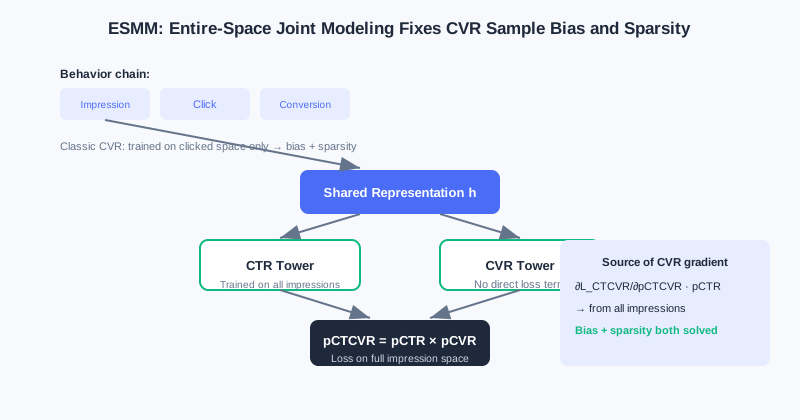
ESMM trains CTR and CVR towers together, computing the Loss with over the entire impression space so that CVR gradients also come from the full samples, resolving bias and sparsity.
Analysis: ESMM/ESM2's "entire-space modeling" cleverly uses product relations to pull dependent objectives back into the same training space — the standard solution for task dependencies. Limitations: it assumes CTR and CVR share the bottom (which can be replaced with MMoE/PLE for a stronger base), and it relies on the business assumption that "the chain decomposes into a product of probabilities."
3.4.4 Multi-Objective Loss Fusion
Once the structure is fixed, jointly optimizing multiple losses is a discipline of its own. Naive weighting has three fundamental flaws: magnitude imbalance (CTR loss 0.1–0.5, CVR can reach 2.0+, and the big loss dominates), asynchronous convergence (sparse tasks are slow), and gradient conflict (task gradients cancel when the angle between them exceeds 90°). Three families of adaptive methods dominate:
- Uncertainty Weight (UWL): dynamically re-weights by per-task (learnable) uncertainty : . A large, uncertain loss gets its weight suppressed, preventing one task from dragging the model off course.
- GradNorm: introduces a gradient loss, dynamically re-weighting by "gradient magnitude " and "relative training rate " so that each task's gradient magnitude and rate tend toward balance, preventing fast tasks from dominating while slow tasks underfit.
- Pareto Optimization: when gradient directions fundamentally conflict (improving A must hurt B), use KKT conditions to make the weights learnable variables, alternately updating parameters and weights (subject to ), steering optimization toward the Pareto frontier (where no solution improves one task without hurting another).
💡 Key Insight: Loss fusion strategies are orthogonal to network structure — whether you use Shared-Bottom, MMoE, or PLE, you can wrap UWL / GradNorm / Pareto around the outside to balance multiple losses. Structure solves "representation conflict"; loss fusion solves "optimization conflict."
⚠️ Common Mistakes in 3.4
| # | Mistake | Example | Why It's Wrong | Fix |
|---|---|---|---|---|
| 1 | Assuming a shared bottom is always beneficial | "Always use Shared-Bottom for multi-task — it's the cheapest" | Hard sharing under task conflict causes negative transfer (seesaw) | Switch conflicting tasks to MMoE / PLE |
| 2 | Confusing MMoE's and PLE's isolation levels | "MMoE already fully separates experts" | MMoE is soft isolation; experts remain visible to all gates | PLE uses CGC to physically separate task experts |
| 3 | Computing Loss directly on the CVR tower | "ESMM trains CVR just like MMoE" | That reintroduces sample selection bias and sparsity | ESMM computes over the entire space with |
| 4 | Hand-fixing loss weights | "w_ctr=1, w_cvr=1 is fine" | Magnitudes / convergence speeds differ; the big loss dominates | Use UWL / GradNorm / Pareto adaptively |
Chapter Summary
📌 Key Takeaways
| Concept | Key Points | Why It Matters |
|---|---|---|
| Negative transfer / seesaw | gradient conflict | The fundamental risk of hard sharing in multi-task learning |
| Shared-Bottom | Shared layers + task towers, parameter-efficient | Good for related tasks; negative transfer under conflict |
| MMoE multi-gate | Per-task dedicated gates pick experts; gradient isolation | Soft isolation eases conflicts |
| PLE / CGC | Shared experts + task experts physically separated | Hard isolation, rooting out interference pathways |
| ESMM entire space | Resolves CVR bias + sparsity | |
| Loss fusion | UWL / GradNorm / Pareto | Solves optimization-level conflicts |
❓ FAQ
Q1: Should I use Shared-Bottom, MMoE, or PLE?
A: Highly related tasks → Shared-Bottom suffices and saves resources; weakly related, conflicting tasks → MMoE; strongly conflicting tasks or when stability is required → PLE. In essence: "the stronger the conflict, the harder the isolation."
Q2: Must ESMM be used together with MMoE?
A: No. ESMM is the "entire-space probabilistic modeling" idea; the original paper's base can be a simple Shared-Bottom, which can also be replaced with MMoE/PLE for stronger bottom representations. The two are orthogonal.
Q3: Which matters more, loss fusion or structure choice?
A: Both matter and they complement each other. Structure decides "whether representations can separate conflicts"; loss fusion decides "whether multiple losses can be optimized in balance." In practice, fix the structure first, then tune the loss-fusion strategy.
🔗 Connections to Later Chapters
- 3.5 (Multi-Scenario) swaps "multi-task differences" for "multi-scenario distribution differences"; multi-tower / dynamic weights share ancestry with the MMoE idea.
- DIN and other models from 3.3 (Sequence Modeling) often serve as the underlying backbone of multi-objective models.
- Part 4 re-ranking optimizes list-level experience on top of ranking (multi-objective scoring); multi-objective scores are the input to re-ranking.
Practice Problems
Work through all problems in order — they get progressively harder. Each has a complete solution you can reveal after trying it yourself.
Problem 3.4.1 — Spotting Negative Transfer 🟢 Easy
A content app simultaneously optimizes "consumption depth (reading time)" and "ad exposure volume." Engineers find that after raising ad exposure, reading time drops noticeably. Is this negative transfer? Explain the mathematical cause.
💡 Solution (click to reveal)
Approach: Check for the seesaw signature of "improving one objective harms the other," and explain via gradient conflict.
Yes, it is negative transfer. The two objectives are negatively correlated, and the shared layer's gradients point in opposite directions: . Shared-Bottom's hard sharing makes the parameter update directions contradictory — optimizing one must hurt the other, falling into a zero-sum game.
Key points:
- Seesaw = hard-sharing conflict between negatively correlated objectives.
- Fix: switch to MMoE/PLE to isolate the conflicting pathways.
Problem 3.4.2 — MMoE vs PLE 🟢 Easy
Judge whether each statement is true or false, and correct it:
- (a) In MMoE each task has a dedicated gate, so there is no gradient interference between tasks anymore.
- (b) In PLE's CGC, task 's gate can also see task 's dedicated experts.
💡 Solution (click to reveal)
Approach: Grasp the "soft vs hard isolation" distinction.
- (a) False: MMoE is soft isolation — experts remain visible to all gates, and even if ignored, gradients may still flow through them during backprop (a latent pathway). Only PLE physically separates.
- (b) False: CGC hard-constrains task 's gate input to be only "shared experts + its own dedicated experts"; it cannot see other tasks' dedicated experts at all, and task 's gradient never updates task 's dedicated experts.
Key points:
- MMoE = soft isolation; PLE/CGC = hard isolation.
- Isolation increases progressively: Shared-Bottom < MMoE < PLE.
Problem 3.4.3 — ESMM's Motivation 🟡 Medium
Why does the traditional CVR model run into problems when "trained on clicked samples, predicting on all impressions"? How does ESMM solve it with ?
💡 Solution (click to reveal)
Approach: Start from the two angles: mismatched sample spaces + sparsity.
A traditional CVR model trains only on clicked samples (CTR positives) but must predict on all impressions online — the training and serving distributions differ → sample selection bias, hurting generalization; and converted samples are extremely sparse (impressions × CTR × CVR), making learning hard.
ESMM trains the CTR and CVR towers together, but instead of computing a Loss on CVR directly, it computes over the entire impression space with . The CVR tower's gradient then flows through from all impression samples — both bias and sparsity are resolved. CVR learns well by indirectly borrowing CTR's full data.
Key points:
- Root cause of the bias: training space (clicks) ≠ serving space (impressions).
- Fix: the product relation pulls CVR back into the entire space.
Problem 3.4.4 — Proving Gradient Conflict in Negative Transfer 🔴 Hard
Let shared parameters serve tasks 1 and 2, with loss changes approximated by . Suppose we apply unified gradient descent , and it is known that (angle greater than 90°). Prove: at least one task's loss must increase.
💡 Solution (click to reveal)
Approach: Substitute and inspect each task's loss change.
. Since , the second term is positive and cancels part of the first term's decrease; if , then and task 1's loss rises. Symmetrically for task 2. Since the two gradients oppose each other, a unified update direction cannot decrease both simultaneously — one side must suffer. That is the mathematical essence of the seesaw / negative transfer.
Key points:
- Opposing gradients → the shared parameter update direction faces a dilemma.
- This explains why MMoE/PLE isolation, or Pareto optimization for non-deteriorating solutions, is needed.
🏆 Challenge: Design a Multi-Objective Solution
An e-commerce platform must optimize three objectives — CTR, CVR, and average order value — where CTR and CVR have a dependency (ESMM-style), and CVR and order value often conflict (seesaw). Combine suitable structures and justify your design (within 150 words), and specify the loss-fusion strategy.
💡 Hint
Use PLE/CGC at the bottom to isolate the CVR / order-value conflict (hard isolation); handle the CTR–CVR dependency with an ESMM-style product jointly in the entire space (the CTR/CVR towers can sit in a shared bottom). At the loss level, use GradNorm or UWL to adaptively balance the magnitudes and convergence speeds of the three losses.
Multi-Scenario Modeling
📝 Before You Continue: Recommended: finish 3.4 Multi-Objective Optimization first. Multi-scenario and multi-task modeling look alike but differ at heart — multi-task handles multiple objectives in one scenario, while multi-scenario handles one objective across different scenarios; both rest on the design philosophy of "sharing + differentiation."
3.4 solved the multi-task problem of "predicting multiple objectives for the same sample." But industrial recommendation often faces multiple scenarios: one app may have home-feed recommendations, search result pages, and "guess you like" below the shopping cart — these scenarios have different data distributions yet must predict the same objective (e.g., CTR). This is multi-scenario modeling.
Training an independent model per scenario ignores cross-scenario commonality, leaves small scenarios data-starved and poorly performing, and multiplies resource costs; mixing all samples into one model ignores scenario differences and hurts accuracy. In this chapter we go from "multi-tower structures" (HMoE, STAR) to "dynamic-weight modeling" (PEPNet, APG, M2M), and see how to balance scenario commonality against scenario specificity.
After reading this chapter, you will be able to:
- Distinguish the essential difference between multi-task (multiple objectives in one scenario) and multi-scenario (one objective across different scenarios)
- Explain how HMoE uses multi-experts + multi-scenario towers + cross-scenario fusion (with stop-gradient) to model commonality
- Explain how STAR uses "star-topology FCN + partitioned normalization + an auxiliary network" to model shared and private parameters together
- Describe how PEPNet's EPNet/PPNet use dynamic gating (Gate NU) to modulate shared parameters
- Work through 4 leveled practice problems comparing the two routes of multi-scenario structures: "physical isolation" vs "dynamic modulation"
3.5.0 Motivation: Multi-Task ≠ Multi-Scenario
First, clear up a common confusion:
- Multi-task learning: same sample, same scenario, predicting multiple different objectives (e.g., one sample gets both CTR and CVR).
- Multi-scenario modeling: different scenarios, different distributions, predicting the same objective (e.g., each scenario predicts its own CTR).
The former is "multiple objectives for one sample"; the latter is "the same objective for different samples." With independent per-scenario models, commonality is ignored (small scenarios suffer, resources explode); with one model trained on mixed samples, differences are ignored (accuracy drops).
💡 Key Insight: The core tension of multi-scenario modeling is — how to share bottom-layer parameters (capturing commonality) while letting the model perceive scenario differences (capturing specificity). This chapter has two routes: ① multi-tower structures (physically isolating some parameters); ② dynamic weights (shared parameters + scenario/sample modulation).
🧠 Mental Model: Chain Stores vs Central Kitchen
Think of multiple scenarios as a company's multiple stores. ① The multi-tower structure is like "each store has its own kitchen (scenario tower) but shares semi-finished products from a central kitchen (shared experts)." ② Dynamic weights are like "all stores use the same central kitchen, but each has a 'flavor adjuster' (Gate NU) that fine-tunes the same dishes to local tastes." The former separates kitchens; the latter adjusts flavors.
3.5.1 Multi-Tower Structures: HMoE and STAR
HMoE (Hierarchical Mixture-of-Experts) borrows from MMoE: the bottom has multiple experts extracting features shared across scenarios, and the top consists of multiple scenario towers (rather than task towers). For scenario , the bottom fuses experts through a gate to get , and the final score fuses the outputs of multiple scenarios:
The key: when fusing other scenarios' scores, stop-gradient blocks their gradient backpropagation — preventing scenario 's samples from directly modifying scenario 's parameters and preserving scenario awareness. Scenario thus uses its own tower while borrowing other scenarios' scores as reference, without mutual pollution.
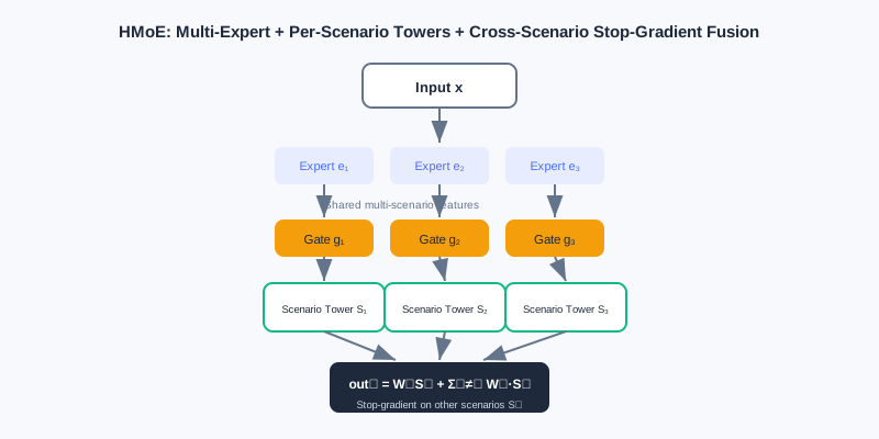
HMoE's bottom experts extract cross-scenario shared features, and each scenario has a dedicated tower on top; when fusing other scenarios' scores, stop-gradient blocks gradients — borrowing commonality without mutual pollution.
STAR (Star Topology Adaptive Recommender) uses a star topology to model shared and private parameters together. Its STAR FCN fuses each scenario's layer parameters as an element-wise product of "shared + private":
where are the scenario-private and globally shared parameters. STAR has two more innovations: Partitioned Normalization (PN) — computing Batch Norm statistics (mean/variance) per scenario (avoiding cross-scenario statistical confusion); and an auxiliary network — feeding scenario features through a shallow network to get auxiliary logits added to the main trunk: .
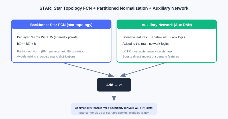
STAR's star FCN fuses "shared center × scenario-private" as an element-wise product, plus partitioned normalization (per-scenario statistics) and an auxiliary network — distinguishing scenarios at both the parameter and normalization levels.
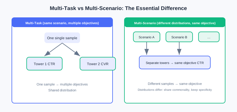
Left: multi-task — same sample, multiple objective towers. Right: multi-scenario — samples from different scenarios, same objective tower; the challenge is sharing commonality while preserving differences.
Analysis: Multi-tower structures (HMoE/STAR) preserve scenario specificity with "physically isolated partial parameters" — intuitive and interpretable. HMoE's stop-gradient prevents scenario pollution; STAR's star FCN + PN separate scenarios at both the parameter and normalization levels. The cost: parameters grow with the number of scenarios (one tower / private parameters per scenario).
3.5.2 Dynamic-Weight Modeling: PEPNet
Multi-tower keeps specificity by "separating kitchens," but shares parameters poorly. PEPNet (Parameter and Embedding Personalized Network) flips the approach: the core network parameters are shared across scenarios, but their behavior is "modulated" through dynamically generated weights that are highly scenario/sample-specific — equivalent to injecting context into the shared network.
The core of PEPNet is the lightweight gating unit Gate NU (inspired by LHUC from speech recognition), which generates dynamic scaling weights with a two-layer network:
The output is dimension-aligned with the target parameters and modulates them via element-wise multiplication . PEPNet uses two modules for layered personalization:
- EPNet (scenario-aware Embedding personalization): feeds scenario priors through Gate NU to generate the gate , then multiplies element-wise with the shared embedding to get scenario-personalized embeddings . Note the stop-gradient applied to the shared embedding, leaving bottom-level learning undisturbed.
- PPNet (user-aware parameter personalization): takes user/content/author ID priors + EPNet's scenario embedding as input, generates per-layer, per-task-tower gates , and modulates every layer's output of the task-tower DNN: . This is sample-level (not task-level) personalization, easing the multi-task seesaw.
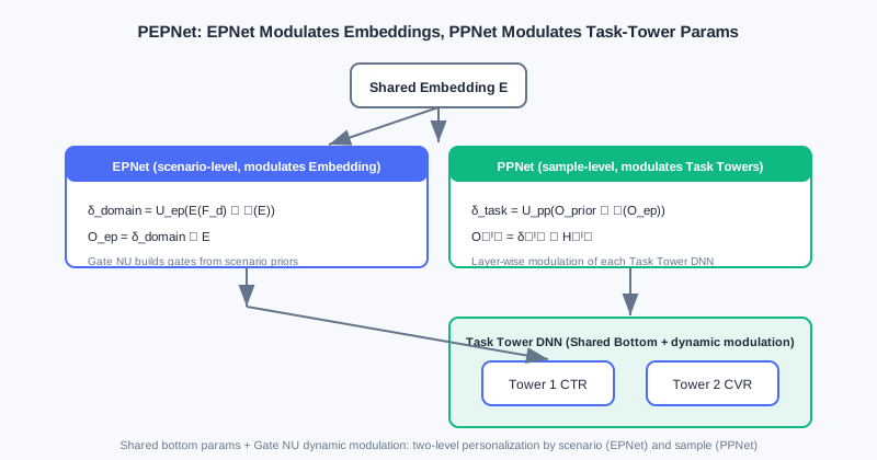
Gate NU generates dynamic scaling weights from scenario/user priors; EPNet modulates the shared embedding (scenario personalization), PPNet modulates each task tower's DNN (sample personalization), while the bottom stays shared.
3.5.3 Dynamic Parameter Generation: APG and M2M
APG (Adaptive Parameter Generation) goes further: it directly generates the parameters for a given sample from that sample. The sample-aware input is reshaped by an MLP into a parameter matrix , and the prediction is . To control cost, APG uses low-rank factorization: , where the private factor is generated from the sample and the shared factors are fixed; the forward pass uses the factored computation to reduce complexity. The shared capture commonality, the private captures specificity — balancing capacity and efficiency.
M2M (meta-learning for multi-scenario multi-task) uses a meta-learner (an MLP) to dynamically generate the task model's parameters from scenario/input features. The backbone contains expert representations , task representations , and a scenario representation ; the meta-learner unit turns the scenario representation into per-layer dynamic parameters applied to features (like an MLP injected with scenario information). It also applies meta-learner units in expert fusion (an Attention meta-network that introduces the scenario during fusion) and in the multi-task towers (Tower meta-networks in a residual style), achieving fine-grained scenario adaptation.
💡 Key Insight: The two routes of multi-scenario modeling converge — multi-tower structures preserve specificity with a "physically isolated parameter space" (divide and conquer); dynamic weights / parameter generation preserve specificity with "shared backbone + dynamic modulation" (injecting context). The latter is more parameter-efficient and flexible, but demands more from the design of the modulation / generation mechanism.
⚠️ Common Mistakes in 3.5
| # | Mistake | Example | Why It's Wrong | Fix |
|---|---|---|---|---|
| 1 | Treating multi-scenario as multi-task | "Multi-scenario is just multi-task with a new name" | Multi-scenario = different distributions, same objective; multi-task = same distribution, multiple objectives | First ask "do the sample distributions differ?" |
| 2 | Fusing HMoE without stop-gradient | "Just add cross-scenario scores directly, gradients flow too" | Scenario a's samples would modify scenario b's parameters, polluting awareness | Add stop-gradient to other scenarios' scores |
| 3 | Missing PN's motivation in STAR | "Global BN statistics are fine" | Mixed multi-scenario samples are not i.i.d. | Use partitioned normalization with per-scenario statistics |
| 4 | Confusing EPNet with PPNet | "Both modulate the task towers" | EPNet modulates embeddings (scenario-level); PPNet modulates towers (sample-level) | EPNet = scenario-level, PPNet = sample-level |
Chapter Summary
📌 Key Takeaways
| Concept | Key Points | Why It Matters |
|---|---|---|
| Multi-scenario vs multi-task | Different distributions, same objective vs same distribution, multiple objectives | Identify the problem type before modeling |
| HMoE multi-tower | Multi-experts + scenario towers + cross-scenario stop-gradient fusion | Shares commonality, preserves scenario awareness |
| STAR star topology | Shared ⊗ private parameters + partitioned normalization + auxiliary network | Separates scenarios at both parameter and normalization levels |
| PEPNet | Gate NU dynamic modulation: EPNet (Embeddings) + PPNet (towers) | Shared backbone + dynamic personalization |
| APG / M2M | Sample/scenario dynamic parameter generation (meta-learning) | Most flexible, parameter-efficient |
❓ FAQ
Q1: When to use multi-tower, and when dynamic weights?
A: Few scenarios with big differences and a need for strong interpretability → multi-tower (HMoE/STAR); many scenarios, parameter-efficiency sensitivity, and fine-grained sample personalization → dynamic weights (PEPNet/APG/M2M). The two can also be combined.
Q2: Why does STAR's star FCN use an element-wise product?
A: makes each scenario's final parameters "shared center × scenario increment" — inheriting commonality while carrying specificity; multiplication (rather than mere addition) lets the private parameters "amplify/suppress" the shared ones as modulation.
Q3: Why does PEPNet's EPNet apply stop-gradient to the shared embedding?
A: To prevent the scenario-personalization gate branch's backpropagated gradients from corrupting the bottom-level shared embedding's general learning — decoupling "commonality" from "scenario differences."
🔗 Connections to Later Chapters
- In 3.4 (Multi-Objective), the MMoE/PLE idea evolves in multi-scenario settings into HMoE's multi-experts + multi-towers; PEPNet's PPNet simultaneously eases the multi-task seesaw.
- Part 4 re-ranking optimizes list-level experience on top of ranking (multi-scenario, multi-objective scoring).
- The end-to-end architectures of generative recommendation (in the next volume) can be seen as a further unification of "multi-scenario / multi-task towers."
Practice Problems
Work through all problems in order — they get progressively harder. Each has a complete solution you can reveal after trying it yourself.
Problem 3.5.1 — Multi-Task or Multi-Scenario? 🟢 Easy
Decide whether each case is "multi-task" or "multi-scenario," and explain why:
- (a) The same home-feed recommendation stream predicts both click-through rate and conversion rate for one sample.
- (b) Two differently distributed traffic sources of the same app — "home feed" and "search results page" — each predicting click-through rate.
💡 Solution (click to reveal)
Approach: Ask "are the sample distributions the same, and are the objectives the same?"
- (a) Multi-task: same scenario (home feed), same distribution, predicting multiple different objectives (CTR, CVR).
- (b) Multi-scenario: different distributions (home vs search), different samples, predicting the same objective (CTR).
Key points:
- Multi-task = same distribution, multiple objectives; multi-scenario = different distributions, same objective.
- Both rely on "sharing + differentiation," but the differentiation targets "objectives" vs "distributions."
Problem 3.5.2 — HMoE's stop-gradient 🟢 Easy
HMoE applies stop-gradient when fusing other scenarios' scores. Briefly state: what goes wrong without stop-gradient?
💡 Solution (click to reveal)
Approach: Think from the angle of "scenario parameter pollution."
In HMoE's fusion formula, the other scenarios' carry stop-gradient to block gradient backpropagation. Without it: scenario 's samples participate in scenario 's score fusion during the forward pass, so during backprop gradients flow along the fusion path and modify scenario 's tower parameters — scenario 's representation gets disturbed by scenario 's samples, the model's scenario awareness degrades, and multi-scenario performance drops.
Key points:
- stop-gradient isolates cross-scenario gradients, preserving "each scenario affects only its own parameters."
- This is the key to HMoE borrowing other scenarios' information without mutual pollution.
Problem 3.5.3 — STAR's Innovations 🟡 Medium
Compared with "independently training one model per scenario," what sharing designs does STAR make to balance commonality and specificity? List at least two and explain their roles.
💡 Solution (click to reveal)
Approach: Recall STAR's three innovations.
- Star FCN: — each scenario's parameters = shared center × scenario-private, inheriting commonality while carrying specificity, avoiding fully independent models.
- Partitioned Normalization (PN): computes BN's mean/variance per scenario, avoiding the statistical confusion caused by non-i.i.d. mixed multi-scenario samples.
- Auxiliary network: scenario features pass through a shallow network to produce auxiliary logits added to the main trunk, strengthening the direct influence of scenario features on the output.
Key points:
- Commonality comes from shared / PN's shared parameters; specificity from / PN's per-scenario statistics.
- Saves parameters versus independent models, and small scenarios can borrow commonality.
Problem 3.5.4 — Small Scenarios and Star Sharing 🔴 Hard
STAR uses : each scenario's private parameters fused by element-wise product with the globally shared . If a scenario has very little data, its private parameters easily overfit. Using the star structure, explain why the shared center alleviates this problem, and describe PN's (partitioned normalization) additional role in this setting.
💡 Solution (click to reveal)
Approach: Look from two angles: "small private parameter count, constrained by sharing" and "normalization stability."
- The final parameters are : although the private overfits easily on few samples, it only performs "amplify/suppress" modulation of the shared center , and the main capability still comes from the data-rich shared . The private parameters are relatively small in dimension and multiplicatively constrained by the shared ones, so their overfitting influence is diluted — sharing acts as regularization.
- PN computes BN's mean/variance per scenario. If a small scenario were mixed into globally pooled batches, its statistics would be dominated by large scenarios and normalization would be unstable; PN lets the small scenario use its own statistics, training more stably and further easing representation shift under few samples.
Key points:
- Star topology = shared fallback + private fine-tuning, naturally resistant to small-scenario overfitting.
- PN adds distribution-level scenario isolation.
🏆 Challenge: Pick a Route and Defend It
A platform has 6 different scenarios (home feed / search / shopping cart / channel pages / push notifications / feed stream), all predicting CTR, with 3 scenarios having very little data. The team has limited resources and wants parameter efficiency without small scenarios collapsing. Choose the "multi-tower" or "dynamic weights" route and justify it (within 150 words), and name a concrete model you could build on if you choose dynamic weights.
💡 Hint
6 scenarios, parameter-sensitive, weak small scenarios → choose the dynamic weights route: shared backbone + dynamic modulation, parameter-efficient, with small scenarios borrowing shared commonality instead of collapsing. You could build on PEPNet (Gate NU modulating embeddings and towers) or APG (sample-wise dynamic parameter generation); multi-tower grows parameters linearly with scenario count at 6 scenarios, and small scenarios' independent towers easily underfit.
When a ranking model emits a list sorted by descending CTR, you often see an awkward phenomenon: the head of the list is dominated by items of the same category and the same style. Ranking pursues point-wise accuracy, but what users want is a great experience across the whole screen. This part stands at the very end of the three-stage funnel — re-ranking — and studies how to bridge the gap where "the highest-scoring list ≠ the best-experience list."
We take two routes. One is the greedy-based family of lightweight rule methods (MMR, DPP): intuitive, interpretable, and easy to deploy. The other is the personalization-based family of data-driven methods (PRM, PRS), which use models to automatically learn the high-order mutual influence among items.
What This Part Covers
| Section | Topic | The Big Idea |
|---|---|---|
| 4.1 | Greedy-based re-ranking | MMR trades off relevance and diversity with a linear combination; DPP uses a determinant framework for more precise control of diversity |
| 4.2 | Personalized re-ranking | PRM models item mutual influence with a Transformer; PRS directly optimizes the experiential gain of permutations |
What You'll Be Able to Do After This Part
- 🟢 Explain why homogenized ranking output is the fundamental motivation for re-ranking, and the two kinds of cost it incurs
- 🟢 Write out MMR's marginal gain formula, and hand-compute a top-k list on a given similarity matrix with the greedy procedure
- 🟡 Derive the DPP kernel matrix , and articulate how the determinant measures diversity
- 🟡 Distinguish the essential difference between MMR (heuristic linear combination) and DPP (precise determinant control) in diversity modeling
- 🔴 Describe how PRM achieves end-to-end list re-ranking with a Transformer plus personalized vectors (PV)
- 🔴 Understand why PRS introduces permutation-variant influence, and how its PMatch / PRank two-stage design resolves the combinatorial explosion
- Complete 8 leveled practice problems to consolidate the core methods of the two chapters
Core Concepts
| Concept | Section | Relevance |
|---|---|---|
| List homogenization / diversity | 4.1 | The reason re-ranking exists: breaking up head repetition and protecting the long tail |
| MMR (Maximal Marginal Relevance) | 4.1 | The most classic and most deployable greedy diversity re-ranking |
| DPP (Determinantal Point Process) | 4.1 | Precisely models set-level diversity through the geometric meaning of the determinant |
| PRM (Personalized Re-ranking Model) | 4.2 | Learns item mutual influence end-to-end with a Transformer |
| PRS (permutation-based re-ranking) | 4.2 | Directly optimizes the experiential gain brought by ordering |
Prerequisites
- You have read the scoring function in Part 3 Ranking and understand how the ranking stage outputs a candidate list with relevance scores
- Some matrix basics (determinants, positive semi-definiteness, Cholesky decomposition) will help you fully digest the DPP derivation
- Familiarity with the Transformer self-attention mechanism will help you understand the PRM encoding layer
- Basic Python and vector representation knowledge
This part is the last link of the three-stage pipeline — we recommend building the full "retrieval → ranking → re-ranking" picture from Parts 1–3 first.
Tips for This Part
- Motivation first, formulas second. Every method in this part exists to solve a "list-level experience" problem; learning formulas detached from their motivation is an easy way to get lost.
- Work the examples by hand. The MMR hand-computation table and the DPP kernel matrix construction in 4.1 — push them through yourself once; it sticks better than ten readings.
- Compare the two routes. After finishing 4.2, look back and compare: greedy methods rely on "hand-crafted objective functions," while personalized methods rely on "models learning from data."
- Remember the visualizations. The accompanying SVGs and interactive HTML in this part turn abstract formulas into observable processes — watch them often and drag the sliders.
Let's dive in! 🚀
Greedy-Based Re-ranking
📝 Before You Continue: Please finish the scoring function in Part 3 Ranking first, and understand how the ranking stage outputs a relevance score (e.g., a predicted CTR) for every candidate. This chapter stands right after that stage, optimizing the "score-sorted" list on its last mile.
Picture this: the ranking model confidently hands over a list whose top ten entries are ten nearly identical "sci-fi action movies." Judged position by position, every score is high and every item is relevant; but stitched into a single list, users immediately feel aesthetic fatigue. This is the real pain point re-ranking addresses — homogenized ranking output.
Re-ranking sits at the very end of the "retrieval → ranking → re-ranking" funnel. Its job is not to recompute accuracy one more time, but to answer a trickier question: holding relevance steady, how do we make the whole list deliver the best experience? Greedy algorithms — with their intuitive ideas, efficient computation, and easy implementation — have become a first-choice strategy for diversity, novelty, and similar problems at the re-ranking stage. They usually do not depend on complex model training; instead, working from predefined rules or objective functions, they build the final list by repeatedly taking the current best option (greedy selection).
This chapter takes a deep dive into two classic greedy re-ranking algorithms: Maximal Marginal Relevance (MMR) and the Determinantal Point Process (DPP).
After reading this chapter, you will be able to:
- Explain the "homogenization" phenomenon in ranking output, and the two kinds of cost it inflicts on user experience and ecosystem efficiency
- Write out MMR's marginal gain formula, and hand-compute a top-k list on a given similarity matrix with the greedy procedure
- Describe how DPP measures set-level diversity with the geometric intuition that "determinant = volume"
- Derive the DPP kernel matrix , and articulate how the relevance term and the diversity term are fused
- Distinguish the essential difference and applicable scenarios of MMR (heuristic linear combination) versus DPP (precise control in a determinant framework)
- Complete 4 leveled practice problems to consolidate hand-computation and code implementation of the two algorithms
4.1.0 Motivation for Re-ranking: Homogenized Ranking Output
The goal of a ranking model is usually to maximize point-wise accuracy (e.g., predicted CTR). When its output is sorted by descending score, the head items tend to be highly similar — back-to-back products from the same category, videos in the same style, content from the same author. This homogenization is no accident; it is the inevitable by-product of point-wise optimization. It directly causes two major problems:
- Degraded user experience: users develop aesthetic fatigue while browsing, their interest decays faster, and content they might otherwise click gets skipped because they have "seen too much of the same kind."
- Lost system efficiency: high-quality long-tail content is under-exposed, platform ecosystem diversity declines, creator motivation suffers, and the supply side is damaged in the long run.
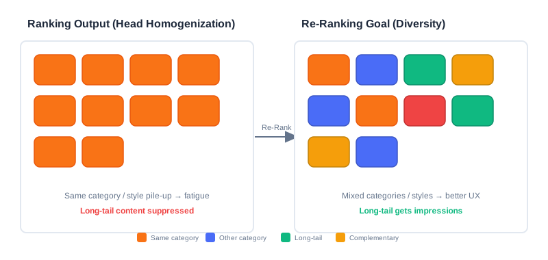
The left side of the figure above is the list the ranking stage spits out directly — ten slots of highly similar content (same-colored blocks clumped together). The right side is the list re-ranking aims to deliver — keeping high relevance while making category, style, and author more varied. The core mission of re-ranking is to break this deadlock of "relevant but repetitive."
💡 Key Insight: What re-ranking pursues is not "Pareto optimality of relevance" but "Pareto optimality of relevance and diversity" — trading a tolerable loss in accuracy for a leap in the experience of the whole list.
🧠 Mental Model: The Buffet Layout
Think of the recommendation list as a buffet spread. The ranking stage is a chef who "picks the most crowd-pleasing dish every time": the result is all braised pork — every plate is popular, but nobody can eat ten plates of meat. Re-ranking is a chef who knows how to compose a menu: while keeping a few signature dishes (high relevance), they interleave cold dishes, soups, and desserts (diversity), so the whole table is tasty without being cloying.
4.1.1 Maximal Marginal Relevance Re-ranking (MMR)
The core goal of MMR (Maximal Marginal Relevance) is to break homogenization by actively introducing diversity while retaining highly relevant items. Its idea is straightforward: each time an item is selected, consider not only how relevant it is on its own, but also penalize how similar it is to the already-selected items.
The Marginal Gain Formula
MMR quantifies the incremental value of item to the current list by defining a marginal gain function:
The symbols mean:
- : the set of already-selected items
- : the relevance score of item , inherited directly from the ranking model's output (e.g., a predicted CTR)
- : the similarity between items and (0~1)
- : the trade-off parameter ()
is MMR's "soul knob":
- : degenerates into pure ranking order (relevance only, no diversity)
- : forces diversity first (possibly at the cost of relevance)
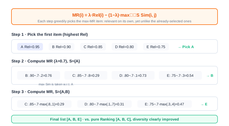
💡 Key Insight: MMR's clever move is defining "diversity" as a similarity penalty against things already selected. The more an item resembles the selected ones, the lower its marginal gain. The greedy process therefore naturally steers away from content that "collides" with what it has already picked.
Sliding-Window Optimization
When the ranking stage produces a large candidate set, computing similarity against all selected items gets expensive. A sliding window offers a targeted optimization: the similarity penalty no longer iterates over the whole , but only over the last selected items (the window ).
where is the last selected items (). The window method sharply cuts computation for long lists and is a common trick in industrial deployments.
Worked Example: Picking top-3 from 5 Items
Suppose the candidate set contains 5 products with their ranking scores (Rel) and the following similarity matrix (the diagonal is 1, meaning full self-similarity):
| Item | Rel | A | B | C | D | E |
|---|---|---|---|---|---|---|
| A | 0.95 | 1.0 | 0.2 | 0.8 | 0.1 | 0.3 |
| B | 0.90 | 0.2 | 1.0 | 0.1 | 0.7 | 0.4 |
| C | 0.85 | 0.8 | 0.1 | 1.0 | 0.3 | 0.6 |
| D | 0.80 | 0.1 | 0.7 | 0.3 | 1.0 | 0.5 |
| E | 0.75 | 0.3 | 0.4 | 0.6 | 0.5 | 1.0 |
Take and walk through the greedy process:
- Initial selection: the highest ranking score A (Rel=0.95); set .
- Round 2 ():
- B:
- C:
- D:
- E:
- Pick B (score=0.57); set .
- Round 3 ():
- C:
- D:
- E:
- Pick E (score=0.405); set .
The final sequence is [A, B, E]. Compared with the pure ranking order [A, B, C], the three items sit in a more varied web of similarity relations, and diversity improves markedly (the source reports a gain of about 37%).
Analysis: MMR's strengths are that it is intuitive, interpretable, and free of training cost, and the knob lets business owners directly tune the relevance-versus-diversity balance. But the costs are clear too: (1) it is a greedy local optimum with no global guarantee; (2) the diversity penalty uses only "the similarity to the single most similar selected item" (max, a pairwise approximation that cannot capture the redundancy when three similar items pile up — exactly the fundamental limitation DPP addresses in the next section.
Code Implementation
def MMR_Reranking(
item_pool, k, lambda_param, sim_func, window_size=None
):
"""Greedy MMR-based re-ranking, with sliding-window optimization."""
candidates = list(item_pool)
S = []
if not candidates:
return S
# Step 1: pick the item with the highest ranking score
first = max(candidates, key=lambda x: x.rel) # ← KEY LINE: the first item must be the most relevant
S.append(first)
candidates.remove(first)
# Step 2: greedy iterative selection
while len(S) < k and candidates:
best_score, best_item = -float("inf"), None
window = S[-window_size:] if window_size and len(S) > window_size else S
for item in candidates:
max_sim = max((sim_func(item, s) for s in window), default=0)
# MMR formula: lambda*Rel - (1-lambda)*max_sim
score = lambda_param * item.rel - (1 - lambda_param) * max_sim # ← KEY LINE
if score > best_score:
best_score, best_item = score, item
if best_item:
S.append(best_item)
candidates.remove(best_item)
else:
break
return S
4.1.2 Determinantal Point Process Re-ranking (DPP)
In the previous section we saw that MMR only computes the pairwise similarity between a candidate and the selected items, greedily steering away from whatever is most similar to them. This approach cannot capture complex repulsion relationships among multiple items (for example, the redundancy of three similar items stacking up), and the determinant captures exactly that, elegantly.
How the Determinant Measures Diversity
Suppose we compute pairwise item similarity via cosine similarity, with each item having a vector representation . For all items to be ranked, , the pairwise similarity matrix follows readily.
Geometrically, a matrix determinant is the "signed volume" of the hyper-parallelepiped spanned by the matrix's column vectors. In the matrix , if the column vectors are linearly dependent (two vectors collinear in 2D, three vectors coplanar in 3D), the vectors "collapse" into a lower-dimensional space and . Conversely, if they are linearly independent, the space they span has no redundancy.
💡 Key Insight: A larger determinant ↔ more "orthogonal" columns ↔ less similar items ↔ higher diversity; a smaller determinant ↔ more collinear vectors ↔ lower diversity. This is the geometric intuition behind measuring diversity with a determinant.
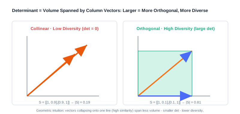
Consider a concrete example. Suppose there are 4 items: a sci-fi action movie, a sci-fi comedy, a costume romance, a costume mystery, with the similarity matrix:
Compare the subsets (both sci-fi) and (sci-fi vs. costume mystery):
Their determinants are:
The results confirm the intuition: crosses genres and is nearly orthogonal — a large determinant (0.81) and high diversity; is same-genre and highly collinear — a small determinant (0.19) and low diversity.
Fusing Relevance and Diversity: The Kernel Matrix
In recommendation, relevance and diversity are both metrics we want. DPP introduces a positive semi-definite kernel matrix to optimize the two together. This matrix decomposes as , where each column of is a candidate item's representation vector. Concretely, each column of is the product of the relevance score (from the ranking stage) and the normalized item vector, so the kernel matrix elements are:
where is exactly the similarity score . The kernel matrix can therefore be written as:
That is, each row and each column of the similarity matrix is multiplied by the corresponding relevance .
🧠 Mental Model: the kernel matrix is a "double-guarantee" score sheet The plain similarity matrix only asks "do they look alike"; the kernel matrix additionally multiplies each item by its own relevance . So an item that is both dissimilar (from what is already selected) and highly relevant (a high score on its own) has the largest "influence" in . Relevance is the admission ticket; diversity is the seating layout — together they determine set quality.
A Kernel Matrix Construction Example
Suppose there are 3 items, with the similarity matrix and the relevance vector :
Computing :
From the Determinant to a "Relevance + Diversity" Objective
For user , with the selected candidate set , the kernel matrix determinant represents set quality:
Taking logarithms on both sides gives:
- The first term concerns only relevance: the larger , the more relevant;
- The second term concerns only diversity: the closer is to orthogonal (cosines near 0), the larger the determinant.
So the objective DPP ultimately optimizes also reduces to the form of a relevance term + diversity term, balanced by the hyperparameter :
Analysis: On the surface, DPP's optimization objective is the same "linear combination of relevance + diversity" as MMR's. But the key difference is this: MMR's diversity penalty looks only at "the pairwise similarity to the most similar selected item" (the max term), a pairwise approximation; while DPP's , through the volume semantics of the determinant, characterizes the mutual repulsion among all items in the subset at once, jointly, and can precisely express the stacked redundancy of three or more similar items.
Greedy Solving: Cholesky Acceleration
DPP is inherently a probabilistic model that converts complex probability computations into simple determinant computations. Inferring the subset that "maximizes " is maximum a posteriori (MAP) inference. The Hulu paper proposed an improved greedy algorithm to solve it quickly: each round, greedily add to the result set the item with the largest marginal gain, until a stopping condition is met:
Since is positive semi-definite, its selected part admits a Cholesky decomposition . After a new item joins, the kernel matrix blocks into:
where and . Using the determinant property of block lower-triangular matrices, we can derive:
So each selection reduces to:
This means each round only needs to maintain and update each candidate's and to pick the best in , avoiding recomputing the whole block determinant — the key to DPP running in real time on industrial-scale candidate sets.
Algorithm flow:
- Initialize: , , , .
- Iterate: while the stopping condition is not met, for each :
- ,
- , update
- Return .
Code implementation:
def DPP_Reranking(item_pool, k, kernel_matrix, epsilon=1e-10):
"""Greedy DPP-based re-ranking (Cholesky-accelerated)."""
n = len(item_pool)
if n == 0 or k <= 0:
return []
cis = np.zeros((k, n)) # stores the c_i vectors
di2s = np.copy(np.diag(kernel_matrix)) # stores d_i^2
selected = []
# Step 1: pick the item with the largest d_i^2 (highest relevance first)
j = int(np.argmax(di2s)) # ← KEY LINE: start from the largest kernel diagonal
selected.append(j)
while len(selected) < k and len(selected) < n:
k_cur = len(selected) - 1
ci_opt = cis[:k_cur, j]
di_opt = math.sqrt(di2s[j])
elements = kernel_matrix[j, :]
# e_i = (L_{ji} - <c_j, c_i>) / d_j
eis = (elements - np.dot(ci_opt, cis[:k_cur, :])) / di_opt # ← KEY LINE
cis[k_cur, :] = eis
di2s -= np.square(eis) # update d_i^2 = d_i^2 - e_i^2
j = int(np.argmax(di2s)) # next, pick the largest log(d_i^2)
if di2s[j] < epsilon:
break
selected.append(j)
return [item_pool[idx] for idx in selected]
def create_kernel_matrix(item_pool, sim_func):
"""Build the DPP kernel matrix L = diag(r) * S * diag(r)."""
n = len(item_pool)
r = np.array([it.rel for it in item_pool])
S = np.eye(n)
for i in range(n):
for j in range(n):
if i != j:
S[i, j] = sim_func(item_pool[i], item_pool[j])
return r.reshape((n, 1)) * S * r.reshape((1, n)) # ← KEY LINE: fuse relevance and diversity
Analysis: DPP's complexity beats "brute-force subset enumeration"; Cholesky acceleration brings each selection down to roughly an update. It controls set-level diversity precisely, and suits scenarios with high diversity-quality requirements and medium candidate sizes (e.g., a final re-ranking over the top 50~200 ranking candidates). The costs: building and maintaining the kernel matrix, sensitivity to similarity quality; and it is still a greedy local optimum with no guarantee of a globally maximal determinant.
The interactive demo below lets you see for yourself: given candidates and similarities, how MMR and DPP pick a list step by step, and how shape the result.
Drag the "trade-off parameter" slider and click "Next" to watch the greedy selection unfold step by step, and compare how MMR's linear penalty and DPP's determinant-volume view lead to different final lists.
4.1.3 MMR vs. DPP: Heuristic Linear Combination vs. Determinant Framework
Having learned both methods, let's nail down their essential differences in one table, to avoid "knowing the formulas but not the distinction."
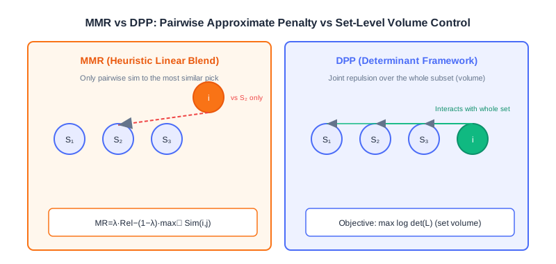
| Dimension | MMR (Maximal Marginal Relevance) | DPP (Determinantal Point Process) |
|---|---|---|
| Diversity modeling | Pairwise similarity to the most similar selected item (the max penalty) | The volume semantics of the whole subset's determinant (joint repulsion) |
| Mathematical essence | Heuristic linear combination: | Determinant framework: measures set quality |
| High-order redundancy | Cannot capture the stacked redundancy of "three collinear items" | Can precisely characterize mutual repulsion among many items |
| Tunability | A single knob , intuitive and easy to grasp | Flexible kernel matrix construction, plus hyperparameter |
| Computational cost | Very low (pairwise similarities) | Medium (kernel matrix + Cholesky acceleration) |
| Best-fit scenarios | Large candidate sets, lightweight and interpretable requirements, fast launches | Medium candidate sets, high diversity-quality requirements |
💡 Key Insight: The two share the same objective shape (a relevance + diversity trade-off) but differ in implementation philosophy: MMR is a heuristic where "humans write the rules and greed executes them"; DPP is a probabilistic framework that "strictly defines diversity through determinant geometry." When your diversity need is only "don't be too repetitive," MMR suffices; when you need precise control of set-level diversity (e.g., exhibition curation, feed deduplication), DPP is the more reliable choice.
🧠 Mental Model: Jigsaw vs. Box-Packing
MMR is like "each time picking the puzzle piece most different from what's already assembled" — it only looks at how the new piece fits the current boundary, a local heuristic. DPP is like "measuring the total volume the whole box of pieces could span before deciding which ones to keep" — it weighs the mutual overlap among all pieces at once, a global measure taken from the set as a whole.
⚠️ Common Mistakes in 4.1
| # | Mistake | Example | Why It's Wrong | Fix |
|---|---|---|---|---|
| 1 | Treating re-ranking as a rerun of ranking | "Can't re-ranking just recompute CTR?" | Ranking seeks point-wise accuracy; re-ranking seeks list-level experience — different objectives | The re-ranking goal is Pareto optimality of relevance × diversity |
| 2 | Setting in the wrong direction | Wanting diversity but setting | degenerates to pure relevance, no diversity | For diversity, lower (e.g., 0.3~0.7) |
| 3 | Believing MMR captures high-order redundancy | Assuming MMR already handles "three similar items" | MMR only uses — it looks at just the single most similar item | Leave high-order redundancy to DPP's determinant |
| 4 | Ignoring similarity quality | Computing Sim on unnormalized features | Similarities outside [0,1] break DPP's positive semi-definiteness and MMR's penalty scale | Normalize first / use cosine similarity |
| 5 | Forgetting to multiply relevance into the DPP kernel | Using only the similarity matrix as | The relevance term is lost; you select "very different but irrelevant" junk | You must use |
Chapter Summary
📌 Key Takeaways
| Concept | Key Points | Why It Matters |
|---|---|---|
| List homogenization | Point-wise optimal ranking → a repetitive head, harming experience and ecosystem | The fundamental motivation for re-ranking |
| MMR | , greedy selection | The lightest, most interpretable diversity re-ranking |
| Sliding window | Penalize only the last selected items | Cuts cost on long lists; common in industry |
| DPP determinant | volume; larger means more orthogonal, more diverse | Rigorously measures set diversity with geometry |
| Kernel matrix | fuses relevance + diversity | Unifies both objectives in one matrix |
| Cholesky acceleration | Pick | Makes DPP feasible in real time |
| MMR vs. DPP | Pairwise approximation vs. set-level precision | Determines method selection |
❓ FAQ
Q1: Must re-ranking come after ranking? Can we do re-ranking alone?
A: Re-ranking's input is "a candidate list that already carries relevance scores," so it inherently depends on ranking (or retrieval) producing candidates first. Doing only re-ranking while skipping ranking amounts to hard-picking from a pool with no quality ordering — the payoff is limited.
Q2: Is the optimal "half relevance, half diversity" setting?
A: Not necessarily. The optimal depends on the business: content communities may lean toward diversity (lower ), while e-commerce search and recommendation may lean toward relevance (higher ). Tune it against online metrics (diversity metrics + retention/duration).
Q3: Is DPP's determinant always better than MMR's result?
A: When you need precise set-level diversity, DPP wins; but MMR is lighter, more interpretable, and easier to tune. For small candidate sets and fast launches, MMR often delivers better cost-effectiveness. There is no absolute winner — it depends on the constraints.
🔗 Connections to Later Chapters
- 4.2 (personalized re-ranking) steps beyond "hand-crafted objective functions," letting PRM/PRS learn list optimality end-to-end from data.
- 3.x (ranking) supplies the relevance scores and the candidates that MMR/DPP need.
- Part 5 trends (debiasing/cold-start): diversity re-ranking is a direct lever against "head concentration and a sunken long tail."
- Generative recommendation (next volume) folds re-ranking into end-to-end sequence generation, replacing MMR/DPP's heuristic objectives with learnable ones.
Practice Problems
Work through all problems in order — they get progressively harder. Each has a complete solution you can reveal after trying it yourself.
Problem 4.1.1 — Spotting the Re-ranking Motivation 🟢 Easy
A short-video app's ranking output has its top 5 entries all being "same-genre skits from the same comedy creator," and users swipe away after watching 2. Identify which problem at the re-ranking stage this reflects, and give one corresponding cost of each kind.
💡 Solution (click to reveal)
Approach: Attribute it with the "homogenization" framework from 4.1.0.
- The problem reflected: homogenized ranking output — point-wise optimization in ranking makes head content highly similar.
- The two costs:
- Degraded user experience: aesthetic fatigue and fast interest decay; users swipe away early (matching the prompt's "swipes away after 2").
- Lost system efficiency: the long tail and other creators' content is under-exposed; ecosystem diversity declines.
Key points:
- The fundamental motivation for re-ranking is to break exactly this "relevant but repetitive" pattern.
- When diagnosing, first separate "insufficient accuracy" from "monotonous experience" — only the latter belongs to re-ranking.
Problem 4.1.2 — Hand-Computing MMR 🟡 Medium
Given 4 candidate items with their Rel scores and similarity matrix (only the upper triangle matters; it is symmetric):
| Item | Rel | A | B | C | D |
|---|---|---|---|---|---|
| A | 0.9 | 1.0 | 0.1 | 0.8 | 0.2 |
| B | 0.8 | 0.1 | 1.0 | 0.3 | 0.6 |
| C | 0.7 | 0.8 | 0.3 | 1.0 | 0.4 |
| D | 0.6 | 0.2 | 0.6 | 0.4 | 1.0 |
Take and use greedy MMR to select the top-3 list (list each candidate's value in every round and the item chosen).
💡 Solution (click to reveal)
Approach: Apply the formula , with .
- Round 1 (S=∅, penalty=0): A: ; B: ; C: ; D: . Pick A (0.54), S={A}.
- Round 2 (S={A}): B: ; C: ; D: . Pick B (0.44), S={A,B}.
- Round 3 (S={A,B}): C: ; D: . Pick D (0.12).
Final top-3: [A, B, D]. Note how C is heavily penalized for being highly similar to A (0.8) — MMR's diversity-driven collision avoidance at work.
Key points:
- Each round only needs the max similarity against the selected set.
- Highly relevant but colliding items (C) get pushed down — exactly the sign that diversity is working.
Problem 4.1.3 — Building the Kernel Matrix 🟡 Medium
Three items have relevance and similarity matrix . Write out the DPP kernel matrix , and state the value and meaning of .
💡 Solution (click to reveal)
Approach: Element-wise, .
- .
- Meaning: the "joint influence" between items 2 and 3 = the product of their relevances × their similarity, fusing relevance and diversity information.
Key points:
- The diagonal is decided purely by relevance (the basis for the initial pick).
- The off-diagonal encodes both "how alike" and "how relevant each is."
🏆 Challenge: Making a Method Selection Argument 🔴 Hard
A feed product has 200 ranking candidates, requires re-ranking latency < 20ms, and the business insists "there must never be 3 consecutive items from the same author." Write an argument for whether MMR (with an added "same-author penalty" rule) or DPP should be preferred. State your trade-offs and the necessary engineering adaptations.
💡 Hint
Weigh latency, controllability, and diversity semantics: with 200 candidates and <20ms, DPP's kernel matrix and Cholesky remain feasible but lean heavy; "no 3 consecutive items from the same author" is a hard business constraint — MMR accommodates rules easily (inject a strong author-dimension penalty into the similarity or penalty term), while encoding the constraint into DPP's kernel matrix is cumbersome. The conclusion usually leans toward MMR + business rules, or DPP with post-hoc constraint enforcement. Argument pivots: interpretability, latency, expressibility of constraints.
Personalized Re-ranking
📝 Before You Continue: Please finish the greedy re-ranking in 4.1 first. This chapter builds on the shared premise that "re-ranking must balance relevance and diversity," but upgrades the means from "hand-crafted objective functions" to "models learning end-to-end from data."
In the previous section we explored greedy re-ranking methods. They make local adjustments to the initial ranked list by explicitly defining optimization objectives for diversity, relevance, or coverage — computationally efficient and highly interpretable. But they fall short when handling complex item-to-item mutual influence and deep personalization:
- The objective functions usually need to be hand-designed, making it hard to capture high-order, non-linear interaction patterns;
- Deeply integrating user personalization information into list-level optimization is also challenging.
This chapter introduces two classic personalized re-ranking models: PRM (Personalized Re-Ranking Model) and PRS (Permutation Retrieve System), to see how models "learn" the optimal list on our behalf.
After reading this chapter, you will be able to:
- Explain why PRM marks the shift of re-ranking from rules/heuristics toward data-driven, end-to-end learning
- Describe PRM's input layer, encoding layer (Transformer), output layer, and how the personalized vector PV is generated
- Write out the self-attention formula, and explain how Softmax implicitly models relative relationships among items in PRM's output layer
- Understand permutation-variant influence, and why PRS optimizes the permutation directly
- Describe PRS's two-stage solution: PMatch (FPSA candidate generation) and PRank (DPWN permutation evaluation)
- Complete 4 leveled practice problems to consolidate the core mechanisms of PRM/PRS
4.2.0 From Rules to Learning: Why Personalized Re-ranking
The diversity objective of greedy re-ranking (MMR/DPP) is "universal" — it applies the same similarity matrix and the same weights to every user. But in real recommendation, the optimal ordering of the same list differs across users: some prefer long-form deep reads first, others prefer short videos; some are price-sensitive, others are not.
This is the founding rationale of "personalized re-ranking": deeply integrating each user's unique preference signals into the optimization of the whole list. It no longer leans on a preset diversity formula; instead, the model learns directly from massive behavioral data "which combination of items, in which order, works best for this user."
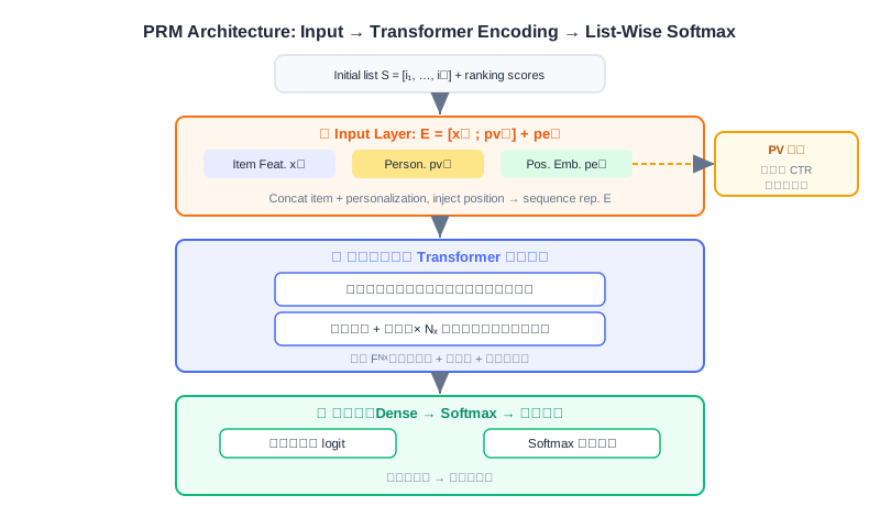
💡 Key Insight: The rule-based approach asks "which list is better on average"; personalized re-ranking asks "which list is better for this user." The former is a population average; the latter gives every individual a list of their own.
🧠 Mental Model: Playlist DJ
Think of greedy re-ranking as a "generic playlist generator" — it only guarantees no repeated genres. Think of PRM as a "DJ who knows you" — he knows that tonight you want slow songs first, then bangers, so he gets the order right too. What the model learns is not "what a playlist should look like," but "what your playlist should look like."
4.2.1 Transformer Personalized Re-ranking Model (PRM)
The introduction of PRM (Personalized Re-Ranking Model) marks an important shift of re-ranking technology from rules/heuristics toward data-driven, end-to-end learning. Its core idea: use the Transformer's powerful sequence modeling to automatically learn the complex mutual influence among items in a list, and deeply integrate fine-grained user personalization into the whole re-ranking process, optimizing globally by maximizing a list-level utility objective (such as click-through rate).
PRM's overall architecture has three layers: the input layer, the encoding layer, and the output layer.
Input Layer: Fusing Personalization and Position
The input layer's core task is to prepare a rich initial representation for each item in the initial list , covering two key aspects:
- The item's own features (): basic information such as item ID embedding, category, tags, and statistical features.
- The user's personalized preference for the item (): encodes the interaction relationship and preference intensity between user and item — the key to PRM's personalization, detailed later.
PRM concatenates the item's raw feature vector with the personalized vector to form a more comprehensive base representation . In addition, the initial list itself carries latent sequential information (higher-ranked items may be more relevant), so a learnable position embedding (PE) is introduced, assigning a vector to each position. The final input representation is:
This combination is usually passed through a simple feed-forward network for dimension adjustment, to fit the Transformer encoder's input.
Encoding Layer: The Transformer Models Item Mutual Influence
The input layer supplies an item sequence carrying personalization and position information. The encoding layer's core goal is to use the Transformer's sequence modeling power to relate all items in the list to one another, capturing their complex, high-order mutual influence. This matters enormously for re-ranking because:
- Whether the user clicks the -th item may be significantly influenced by the -th (or even more distant) item — a substitute, a complement, or a source of variety;
- Such influence is often long-range, unconstrained by items' initial physical positions.
The Transformer's core mechanism is self-attention: every item in the sequence can attend to every other item (including itself), computing the similarity between its query vector and other items' key vectors to obtain attention weights, which decide how much information to aggregate from other items:
PRM adopts multi-head attention, organized in standard Transformer encoder blocks (multi-head self-attention + feed-forward network), stacked in multiple layers that progressively distill higher-order inter-item dependencies. The final output is each item's high-level representation , which fuses item features, personalized user preference, and contextual interaction information across the whole list.
Analysis: Compared with MMR/DPP's "pairwise similarities," PRM's self-attention can model arbitrary high-order, non-linear inter-item dependencies and naturally absorbs user signals. The costs: it needs training data, its inference cost exceeds rule-based methods, and the attention weights are less intuitive than MMR's formula — interpretability drops. It fits core scenarios with abundant data and sensitivity to personalization gains.
Output Layer: Softmax List-Level Scoring
PRM applies a linear transform () to each item's high-level representation , mapping it to a scalar score (logit), then feeds it into Softmax:
Softmax plays two key roles here:
- Normalization: it converts all scores into a probability distribution, with item probabilities summing to 1;
- Implicit relative-relationship modeling: each item's final probability depends not only on its own score but also on its relative comparison against all other items' scores in the list — a natural fit for re-ranking's need to assess items' relative importance.
Generating the Personalized Vector (PV)
Looking back at the whole pipeline, PV is what distinguishes PRM from ordinary re-ranking and makes it truly "personalized." Where does PV come from? PRM adopts a clever and practical strategy: use a pre-trained click-through-rate prediction model to generate PV.
- The pre-trained model's role: trained on massive user behavior history, it learns to predict the probability that user with behavior history clicks candidate item .
- Extracting the personalized vector: PRM does not use the predicted click probability itself, but extracts the hidden-layer activation just before the model outputs the final click probability (usually via Sigmoid). This vector carries rich abstract information about "how much user prefers item ," and serves as item 's personalized vector with respect to user .
- Feeding PRM: for every item in the initial list, is computed through the pre-trained model above and passed as a key input into PRM's input layer.
Core code (excerpt):
# User-side embedding -> [B, max_len, D], so every position carries the same user context
user_part_embedding = tf.tile(tf.expand_dims(user_part_embedding, axis=1),
[1, max_seq_len, 1])
# Page-level sequence representation: concatenate user + item features + PV + item embedding
page_embedding = concat_func(
[user_part_embedding, item_part_embedding, pv_embeddings, item_embeddings],
axis=-1) # ← KEY LINE: fuse four kinds of signals
# Add position encoding to form the Transformer's final input
enc_inputs = add_func([page_embedding, position_embedding]) # ← KEY LINE: inject position information
# Stack Transformer encoder layers
for _ in range(transformer_blocks):
enc_inputs = TransformerEncoder(
intermediate_dim, nums_head, dropout_rate,
activation="relu", normalize_first=True, is_residual=True)(enc_inputs)
# Scoring head: map each position to one probability
enc_output = tf.keras.layers.Dense(intermediate_dim, activation='tanh')(enc_inputs)
enc_output = tf.keras.layers.Dense(1)(enc_output)
score_output = tf.keras.layers.Activation(activation='softmax')(
tf.keras.layers.Flatten()(enc_output)) # ← KEY LINE: list-level relative scoring
The paper's experiments show that PRM delivers consistent gains over baselines on metrics like map@5, validating the effectiveness of end-to-end personalized re-ranking.
The interactive demo below gives you a direct feel for how PRM "reads" through the whole list with a Transformer step by step, then outputs a re-ranked relative probability for each position:
Click "Next" to watch: how the initial list enters the encoder carrying PV and position embeddings, how self-attention progressively aggregates cross-item information layer by layer, and how Softmax finally turns scores into re-ranked relative probabilities.
4.2.2 Permutation-Based Re-ranking Model (PRS)
Although PRM achieves end-to-end personalized re-ranking with a Transformer, it still has one fundamental limitation: a lack of deep understanding of the impact of permutations.
Picture a scene: a user feels no urge to buy when facing the list [A, B, C], yet buys A upon seeing the permutation [B, A, C]. This phenomenon is called permutation-variant influence — one plausible explanation: placing the pricier B up front makes A feel relatively cheap, which triggers the purchase.
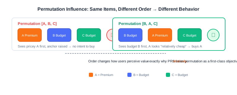
Traditional re-ranking (including PRM) focuses mainly on optimizing individual item scores, while ignoring the influence of the item ordering itself on user behavior. PRS's design idea: evaluate all possible item permutations and pick the one with the best user experience. But items have permutations — computationally infeasible — so PRS proposes a two-stage solution:
- PMatch stage: a search algorithm quickly screens down to a small number of candidate permutations;
- PRank stage: a neural network evaluates these candidates' quality and picks the winner.
The PRS Overall Framework
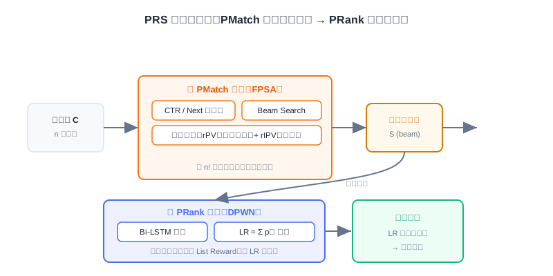
The PMatch Stage: Candidate Permutation Generation (FPSA)
PMatch (Permutation-Matching) aims to efficiently identify candidate permutations from the exponential permutation space. It employs FPSA (Fast Permutation Searching Algorithm), combining beam search with two user-behavior prediction models.
Offline training: a dual-model prediction system
- CTR model: predicts the probability that the user clicks an item,
- Next model: predicts the probability that the user keeps browsing to the next item after finishing the current one,
Both are modeled in the standard point-wise fashion (Sigmoid activation + cross-entropy loss):
The Next model reflects the continuity of user browsing: an item must not only attract clicks but also lead the user on to subsequent content.
Online serving: the FPSA algorithm
FPSA models user browsing as a sequential decision process — an item's value in a sequence depends not only on its own features but also on its role along the whole browsing path. At its core, a beam search builds candidate permutations step by step, pruning by a reward function at each step. The reward fuses two metrics:
- rPV (Page View Reward): measures the total browsing depth a permutation can bring, encouraging combinations that guide users deeper;
- rIPV (Item Page View Reward): measures the total probability of items in the permutation being clicked, securing commercial value.
FPSA core code (excerpt):
def fpsa_algorithm(items, ctr_scores, next_scores, beam_size=5, max_length=10,
alpha=0.5, beta=0.5):
"""Fast Permutation Searching Algorithm (beam search generates candidate permutations)."""
S = [()] # candidate permutation set, initially the "empty sequence"
for i in range(1, max_length + 1):
St = S.copy()
S, R = [], {}
for O in St:
for ci in items:
if ci not in O:
Ot = O + (ci,) # append the unseen item ci to the tail
r = calculate_estimated_reward(Ot, ctr_scores, next_scores, alpha, beta)
R[Ot], S.append(Ot) = r, Ot
# Beam search truncation: keep the top beam_size by reward
S = sorted(S, key=lambda x: R[x], reverse=True)[:beam_size] # ← KEY LINE
return S
def calculate_estimated_reward(O, ctr_scores, next_scores, alpha, beta):
r_pv, r_ipv, p_expose = 1.0, 0.0, 1.0
for ci in O:
p_ctr, p_next = ctr_scores[ci], next_scores[ci]
r_ipv += p_expose * p_ctr # accumulate expected clicks
p_expose *= p_next # exposure-chain probability decays with position
r_pv = p_expose # probability of browsing to the end
return alpha * r_pv + beta * r_ipv # linearly fuse PV and IPV
Analysis: FPSA's beam search cuts down to a manageable candidate set — a pragmatic engineering answer to combinatorial explosion. But it depends on the accuracy of the two point-wise CTR/Next models, and its reward is a linear fusion that may miss non-linear permutation gains.
The PRank Stage: Permutation Evaluation (DPWN)
PRank (Permutation-Ranking) takes the candidate permutations PMatch generates and evaluates each permutation's quality with the neural network DPWN (Deep Permutation-Wise Network).
DPWN's design philosophy: an item's value in a permutation depends not only on its own features but also on its position and role in the context of the whole sequence. To this end it adopts a Bi-LSTM architecture:
- Sequence encoding layer: a bidirectional LSTM computes the contextual representation of the -th item:
- Feature fusion layer: , fusing sequence representations with user/item features.
- Prediction layer: an MLP predicts the click probability of each position, .
List Reward (LR) is PRank's core evaluation metric, defined as the sum of predicted click probabilities over all items in the permutation:
During online serving, PRank computes the LR of every candidate permutation and outputs the permutation with the highest LR.
💡 Key Insight: The fundamental divide between PRS and PRM is this — PRM optimizes "each item's relative score," with positions implied by scores; PRS directly optimizes the experiential gain brought by the ordering itself (LR), treating order as a first-class citizen. The former cares about "which items to pick"; the latter cares about "how to arrange them."
🧠 Mental Model: Shelf Display vs. Item Pricing
PRM is like a manager who prices each product — he gets every tag as accurate as possible, but the shelf order is just sorted by price. PRS is like a store manager who obsesses over display — he knows that "putting the expensive end-of-season piece up front makes the mid-shelf bargain look like a deal," so he optimizes the placement order of the whole product group separately.
⚠️ Common Mistakes in 4.2
| # | Mistake | Example | Why It's Wrong | Fix |
|---|---|---|---|---|
| 1 | Assuming PRM is personalized by default | "PRM can personalize with only item features as input" | Personalization comes from PV; without PV it degenerates into ordinary re-ranking | You must feed in the pre-trained CTR model's hidden layer as PV |
| 2 | Confusing PRM with a ranking model | "PRM is just CTR prediction" | PRM optimizes list-level relative relationships; ranking is point-wise | Remember PRM's output is Softmax relative probabilities |
| 3 | Ignoring permutation-variant influence | "[A,B,C] and [B,A,C] work the same" | Order changes users' relative price/preference perception | Only PRS-style methods treat order as an optimization target |
| 4 | Underestimating the explosion | "Just enumerate all permutations and pick the best" | 10! ≈ 3.6 million; 20! is beyond computation | Use PMatch's beam search to cut candidates |
| 5 | Treating PRS as single-stage | "PRank searches permutations directly" | Without PMatch's candidate generation, PRank has nothing to evaluate | Both stages are indispensable |
Chapter Summary
📌 Key Takeaways
| Concept | Key Points | Why It Matters |
|---|---|---|
| Motivation for personalized re-ranking | Rule methods apply one objective to everyone; no per-user adaptation | Deeply integrates user preference into list optimization |
| PRM input layer | , fusing four kinds of signals | PV is the core of personalization |
| PRM encoding layer | Transformer multi-head self-attention models high-order mutual influence | Captures cross-item, long-range dependencies |
| PRM output layer | Softmax → list-level relative probabilities | Implicitly models relative importance among items |
| PV generation | Take the pre-trained CTR model's hidden-layer activation | Reuses existing ranking knowledge for personalization |
| Permutation-variant influence | Same items, different order → different behavior | The motivation for PRS's existence |
| PRS two stages | PMatch(FPSA+beam)→PRank(DPWN+LR) | Dissolves the combinatorial explosion |
❓ FAQ
Q1: Can PRM be combined with DPP from 4.1?
A: Yes, and it's common. DPP/MMR often serves as a baseline or post-processing for PRM: first let PRM learn list-level preference, then apply DPP as a diversity-constraint safety net. The two are complementary — one handles personalization, the other set diversity.
Q2: Why take the hidden layer for PV instead of the final click probability?
A: The final click probability is a scalar squashed by Sigmoid — heavily compressed information; the hidden-layer activation is a high-dimensional abstract vector that preserves rich semantics about "why the user prefers this item," making it a better personalized input for PRM.
Q3: Can PRS's beam search miss the truly optimal permutation?
A: Yes. The beam keeps only the top- local candidates by reward — it's an approximation. But versus full enumeration, this is a necessary engineering trade-off; in practice, with a good reward function, the top candidates are already high quality.
🔗 Connections to Later Chapters
- 4.1 (greedy re-ranking) is the contrasting baseline for PRM/PRS — rule methods are lightweight; personalized methods are expressive.
- Part 3 ranking supplies the pre-trained CTR model and ranking scores PRM needs — the source of PV.
- Part 5 trends (the generative paradigm) pushes "list generation" further toward end-to-end; PRS's permutation-optimization idea re-emerges naturally as autoregression in generative architectures.
- The next volume on generative recommendation replaces the "retrieval → ranking → re-ranking" cascade with a single sequence model, folding re-ranking's objective directly into the generation objective.
Practice Problems
Work through all problems in order — they get progressively harder. Each has a complete solution you can reveal after trying it yourself.
Problem 4.2.1 — Telling the Two Kinds of Re-ranking Apart 🟢 Easy
Decide whether each description below is closer to (a) greedy re-ranking (MMR/DPP) or (b) personalized re-ranking (PRM/PRS), and explain why:
- (i) The system re-ranks every user with the same similarity matrix and a fixed .
- (ii) The system extracts the pre-trained CTR model's hidden-layer vector for each user as re-ranking input.
💡 Solution (click to reveal)
Approach: Grasp "whether user personalization is incorporated, and whether it is data-driven."
- (i) Greedy re-ranking: fixed similarity and , identical for all users, no personalization — a rule/heuristic approach.
- (ii) Personalized re-ranking (PRM): taking the pre-trained CTR model's hidden layer as PV is PRM's signature move, deeply incorporating user preference.
Key points:
- Whether "per-user personalized signals" exist is the essential dividing line between the two families.
- Presence of PV ≈ PRM; a fixed objective function ≈ a greedy method.
Problem 4.2.2 — PRM's Input Representation 🟢 Easy
In PRM, from which parts is an item 's final input representation assembled by concatenation/addition? Write the formula and explain what problem each part solves.
💡 Solution (click to reveal)
Approach: Recall the input layer of 4.2.1.
Formula:
- concatenation: fuses "what the item is" with "how much the user prefers it" (personalization), solving the per-user-adaptation problem;
- position embedding: injects position information within the list, solving the problem that "the Transformer itself carries no order."
Key points:
- Concatenation merges features from different sources; addition injects position.
- All three parts are indispensable: no PV means no personalization; no PE means no sense of order.
Problem 4.2.3 — Analyzing Permutation-Variant Influence 🟡 Medium
An e-commerce list has items [A (expensive), B (budget), C (budget)]. The product manager finds that changing [A, B, C] to [B, A, C] noticeably lifts A's click-through rate. Explain this phenomenon with "permutation-variant influence," and state what it implies for re-ranking method selection.
💡 Solution (click to reveal)
Approach: Use the permutation-variant influence framework from 4.2.2.
- Explanation: A is the expensive item. When A comes first ([A,B,C]), the user sees the high price first and their threshold rises; after switching to [B,A,C], the user sees the budget B first, and A then feels "relatively cheap," triggering the purchase urge — that is, order changes the user's relative perception of value, which is permutation-variant influence.
- Implication: Traditional point-wise scoring (including PRM's score optimization) assumes "order doesn't affect an item's value" and misses this gain. You need a method like PRS that treats "the ordering itself" as the optimization target (evaluating whole-list gains with LR) to capture the experiential lift brought by order.
Key points:
- Permutation-variant influence = same items, different order → different behavior.
- It points toward methods where "order is a first-class optimization target" (PRS), not methods that only optimize individual item scores.
🏆 Challenge: Designing a Hybrid Re-ranking Scheme 🔴 Hard
A feed product wants both "personalization" (PRM's strength) and "strong set diversity" (DPP's strength), while controlling inference latency. Write a short design argument (within 150 words): how to combine PRM and DPP (in sequence / in parallel / in cascade), and give one risk of each sub-option and a mitigation.
💡 Hint
Three common combinations: (1) Cascade — PRM scores, then DPP does diversity post-processing; the risk is DPP may break the personalized order PRM learned; mitigate with a soft constraint. (2) Parallel — score both ways and fuse with weights; the risk is the weights are hard to tune; mitigate with offline grid search. (3) Inject PV into the DPP kernel — encode PRM's PV into ; the risk is the kernel must be recomputed; mitigate with incremental updates. Focusing your argument on one option is enough.
The earlier parts walked you through the complete industrial chain of discriminative recommendation — retrieval, ranking, re-ranking. But a real recommender system is far more than "ordering candidates well". It must also confront biased data, items and users with no history, and an ongoing paradigm shift: from "scoring every candidate" to "directly generating recommendation sequences".
This part does not add another standalone algorithm module. Instead, it pulls the camera back so you can see the three approaches industry and academia take when correcting, completing, and reshaping recommender systems.
What This Part Covers
| Section | Topic | The Big Idea |
|---|---|---|
| 5.1 | Model debiasing | Data is naturally biased and sits inside a feedback loop; correct it with IPS reweighting and PAL's position decoupling |
| 5.2 | Cold start | Use content, meta-learning, and segmentation architectures to build effective representations for items and users with no history |
| 5.3 | Evolution of the generative paradigm | From discriminative scoring to generative sequence generation — the leap from memorization · generalization to understanding · reasoning |
What You'll Be Able to Do After This Part
- 🟢 Explain where a recommender's data biases come from (selection/exposure/conformity/position) and how result biases (popularity/unfairness) get amplified through the feedback loop
- 🟢 Apply inverse propensity score (IPS) reweighting, and use PAL to decouple position effects from user preference structurally
- 🟡 Compare the different solutions for content cold start (CB2CF / MetaEmbedding) and user cold start (MeLU / POSO)
- 🟡 Describe the three evolutionary paths of generative recommendation: generative retrieval (HSTU / TIGER), generative ranking (GenRank / MTGR), and end-to-end unified generation (OneRec)
- 🔴 Argue, against Part 1's two paradigms, how the discriminative cascaded architecture can be replaced by a generative end-to-end one
Core Concepts
| Concept | Section | Relevance |
|---|---|---|
| Selection bias / exposure bias / position bias | 5.1 | The root of untrustworthy training data; requires active correction |
| Inverse Propensity Score (IPS) | 5.1 | Weighting by for an unbiased risk estimate |
| Position-bias Aware Learning (PAL) | 5.1 | Structurally separating "seeing" from "liking" |
| Content cold start: CB2CF / MetaEmbedding | 5.2 | Letting new items borrow collaborative representations from content |
| User cold start: MeLU / POSO | 5.2 | Serving new users with meta-learning or segmented submodules |
| Semantic IDs / end-to-end generation | 5.3 | The core of generative recommendation: understand content, generate directly |
Prerequisites
- Finish the two paradigms and the three-stage funnel of Part 1 first
- Know the basic models of Part 2 Retrieval and Part 3 Ranking (collaborative filtering, two-tower, matrix factorization)
- Have basic deep-learning and sequence-model concepts (Transformer self-attention; meta-learning/MAML will help with 5.2/5.3)
This part is the bridge that closes out the fundamentals — it patches the defects of the pipeline from earlier parts while pointing toward the generative follow-up volume.
Tips for This Part
- Treat bias as an invisible opponent. While reading 5.1, keep asking: does this training sample really represent the user's true preference?
- The core of cold start is borrowing strength. A new item has no behavior, so borrow content; a new user has no history, so borrow meta-knowledge or population structure.
- 5.3 loops back to Part 1. It grounds "discriminative vs generative" in concrete models (HSTU, TIGER, OneRec).
Let's dive in! 🚀
Model Debiasing
📝 Before You Continue: Make sure you have read the two paradigms and the three-stage funnel in 1.1, and the scoring function in Part 3 Ranking. This chapter adds a layer of realism on top of those "ideal assumptions": the data you train your model on is not clean.
When you prepare to train a recommendation model on massive interaction data, there is a gentle but fatal illusion: "more data, more accurate models". In a real recommender system, data comes from users' free behavior inside a product, not from controlled lab experiments. Every click, rating, and dwell is shaped by countless factors: how the system itself presents items, the user's own habits, and how popular an item already is.
More subtly, recommender systems have a feedback loop: today's recommendations determine what users see tomorrow, and tomorrow's clicks become the samples used to retrain the model the day after. Once this loop starts spinning, a tiny initial bias snowballs. This chapter walks you through these biases and introduces two debiasing toolkits that hold up under causal-inference scrutiny — IPS and PAL.
After reading this chapter, you will be able to:
- Distinguish the two families of bias sources: data bias (selection/exposure/conformity/position) and result bias (popularity/unfairness)
- Explain how the feedback loop amplifies small biases into a Matthew effect of homogeneous recommendations
- Write down the IPS estimator, justify why it is an unbiased estimate of the true risk, and know how to clip weights when they explode
- Use PAL's two-module architecture to structurally decouple "seeing" from "liking"
- Work through 4 tiered practice problems to consolidate the math and engineering intuition of debiasing
5.1.0 Data Is Born Biased: The Feedback-Loop Trap
To understand bias, first accept one fact: the interactions we observe are not the user's true preferences. In a lab you could show users random items and record their reactions, but in a production system users only see the content the system "chose" to show them.
Biases in recommender systems fall into two families depending on when they arise:
- Data bias arises at the data-collection stage and is the root of everything that follows. The model sees a world already filtered by the system.
- Result bias shows up in the recommendations themselves — data bias processed and amplified through model training.
The two are not isolated; they feed each other through the feedback loop. Popular items get recommended more → receive more interactions → take a larger share of the next round of training data → the model favors them even more. This is the rich-get-richer Matthew effect.
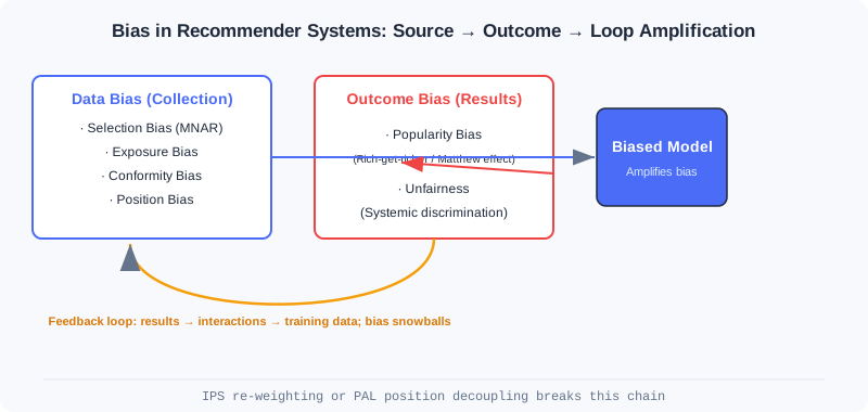
The figure chains "data bias → result bias → feedback loop" together: a biased model is both a product of bias and a factory of even more biased data.
💡 Key Insight: What gets seen is not what is preferred. Debiasing is not about "feeding more data" — it is about re-understanding the mechanism that generated the data. That is the shared starting point of IPS and PAL.
5.1.1 Data Bias: Seeds Sown at Collection Time
Data bias has four typical faces, stemming respectively from user habits, system exposure policy, and social psychology.
Selection bias appears in explicit-feedback (rating) settings. Users tend to rate only content they care about, so the ratings we observe do not represent their true attitude toward all items. Many neutral or negative potential ratings are never recorded — research calls this Missing Not At Random (MNAR). It leads the model to overestimate overall user satisfaction.
Exposure bias is the core challenge of implicit feedback (clicks/watches). Users can only see items the system recommends to them; a non-interacted item can mean one of two things: genuinely not interested (true negative), or never seen at all (potential positive). If you naively treat every "no interaction" as a negative, the model learns distorted preferences — long-tail items suffer most, because they never had much exposure to begin with.
Conformity bias comes from group effects in social psychology. Seeing thousands of positive reviews, users often echo them with positive ratings to seek group approval — and vice versa. The collected feedback is thus not an independent, authentic preference, but an expression contaminated by public opinion.
Position bias is especially visible in list-wise recommendation. Users naturally attend more to items at the top, regardless of relevance. Data shows CTR decays sharply with position — a "click" reflects preference, but is also heavily manipulated by position.
🧠 Mental Model: A Telescope With Filters
Think of training data as a telescope with built-in filters. You observe the universe (true user preferences) through it, but the filters only let through the light of "what the system displayed, what the user happened to click, what sat near the top, what everyone praised". A denser star chart does not mean that region actually has more stars — it may just be filter bias. Debiasing means calibrating the filters.
Analysis: These four biases do not all call for the same treatment. Selection/exposure bias is essentially "unequal observation probability" and suits IPS weighting to compensate at the loss level; position bias has a clear structure — it only affects "whether the item was seen" — so PAL, which decouples it at the architecture level, is the cleaner fix. Diagnose the bias type first, then pick the tool.
5.1.2 Result Bias: The Model Learns the Bias In
When biased data flows through a model, the bias does not vanish; it is often reinforced and shows up in the results.
Popularity bias is the most common result bias. Popular items contribute the vast majority of interactions in training data, the model acquires the habit of "recommend popular, harvest clicks", and ends up recommending them even more frequently than their underlying popularity. This dilutes personalization and robs long-tail items of any chance to be discovered.
Unfairness means the system exhibits systematic discrimination against certain user groups or item categories. If a group kept receiving poor recommendations in historical data, the model learns and perpetuates that prejudice, staying unfair in future recommendations.
⚠️ Warning: Popularity bias and the feedback loop are symbiotic. Popular items get more exposure, hence more interactions, hence a bigger share of the next round of data, which further inflates popularity bias — unless you actively cut this chain in the model or the training loop, it keeps worsening until recommendations become extremely homogeneous.
5.1.3 Correcting Selection Bias with Inverse Propensity Scores (IPS)
Inverse Propensity Score (IPS) originates from causal inference. It treats "showing an item" in a recommender system as an intervention, and removes selection bias through reweighting.
The core idea is intuitive: if a sample is easy to observe in the first place (a hot product, an item in slot 1), its contribution during training should be discounted; conversely, if a sample is hard to observe yet the user found it and interacted with it (a long-tail item, a low-position item), it likely carries a stronger true-preference signal and deserves a higher weight.
The propensity score is the key concept, defined as the probability that the interaction between user and item is observed, . IPS's core operation is to weight by its reciprocal — inverse weighting: high propensity → low weight, low propensity → high weight.
A Concrete Example
Consider a movie recommender with two user groups: horror fans and romance fans. Horror fans rarely rate romance movies on their own (observation probability ), but when they occasionally do, they give genuinely low scores (1–2); they frequently rate horror movies () and give high scores (4–5).
Naively averaging the observed data would show horror movies rated far above romance movies, misleading the model into overestimating the preference gap. With IPS weighting, the rare "horror fan rates romance low" sample gets a × weight while the common "horror fan rates horror high" sample gets only × — the model can now recover the true preference distribution more accurately.
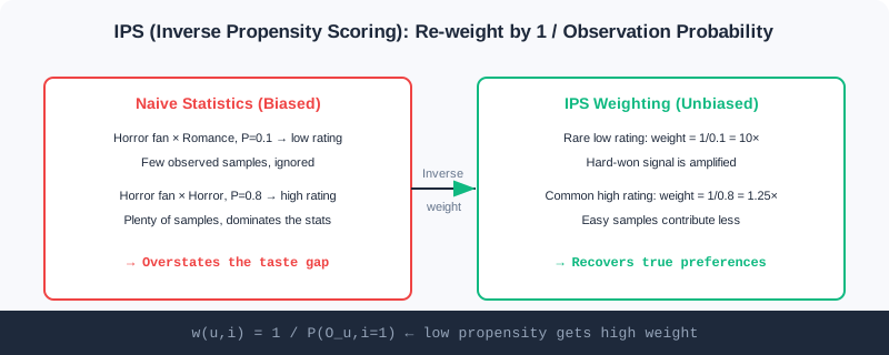
On the right, IPS weighting amplifies the few hard-won low-score samples and discounts the cheap high-score samples, converging toward the true gap.
🧠 Mental Model: Weight Vouchers for Rare Samples
Imagine running a survey where only talkative people agree to be interviewed and the silent rarely speak up. Tallying raw interview counts would drown out the silent group's opinions. IPS is like issuing every silent respondent's statement a 10×-weight voucher — so their voices are heard in proportion to the true population.
The Math Behind IPS
The traditional evaluation approach computes the average loss directly on observed data:
where is the observed dataset, is the true rating, is the predicted rating, and is the loss or evaluation metric. When selection bias exists, — the naive estimator is biased.
The IPS estimator introduces propensity-score weighting:
It can be shown to be an unbiased estimator of the true risk: .
IPS applies not only to evaluation but also to training directly. The traditional matrix factorization objective:
Adding IPS weights just multiplies each sample's loss by :
A tiny change that integrates seamlessly into existing optimizers.
⚠️ Warning: When some samples have extremely small propensity scores (e.g. ), the reciprocal reaches 100×, exploding the estimator's variance and destabilizing training. In practice weights are usually clipped or normalized — trading a bit of "unbiasedness" for lower variance.
Where Propensity Scores Come From: Estimated, Not Given
The key practical challenge for IPS is that propensity scores are usually unknown and must be estimated by an auxiliary model. A Naive Bayes approach assumes the observation probability depends only on the rating value (a 5 is far more likely to be observed than a 1); a logistic regression approach builds a "was it observed" classifier from user/item features, capturing more complex observation patterns and estimating more accurately.
Verifying That Debiasing Works: Semi-Synthetic Experiments
A classic approach is the semi-synthetic experiment, which keeps the complexity of real data while letting us control how severe the bias is:
- Build a true rating matrix: take MovieLens 100K (944,000 ratings, but only 6% of the matrix is filled), and complete it with matrix factorization into a full that serves as ground truth.
- Design a bias model: for a user–item pair with rating , if the observation probability is (a base probability); if it is (decaying). means no bias; the smaller , the heavier the bias; is tuned so the overall observation rate is about 5% to mimic sparsity.
- Generate biased observed data: randomly decide observation according to those probabilities, yielding a biased training set.
- Compare estimators: the true MAE is computed on ; the naive estimator computes average error directly on observed data; IPS computes a weighted average error with weights .
Experiments show that at , the IPS estimator's error is 2–3 orders of magnitude smaller than the naive estimator's. This kind of "known-answer" testbed makes the effect of different debiasing methods precisely measurable, and has become the standard way to validate them.
The interactive demo below gives a hands-on feel for how "naive → IPS" recovers the gap:
Click "Next" or "Autoplay" and watch how the observed average scores of horror and romance movies go from "naive covers up the gap" to "IPS restores the true gap".
Analysis: IPS's strengths are simplicity and generality — a one-line weight change embeds it in any recommender model, with a theoretical unbiasedness guarantee. The price is variance: the more extreme the weights, the shakier the training, so production almost always pairs it with clipping. Moreover, IPS only compensates "unequal observation probability" biases (selection/exposure); for structured problems like position bias it is not the best fit — that is what PAL is for.
5.1.4 Decoupling Position Bias from User Preference with PAL
When users scroll on their phones, are they more likely to tap content near the top? Yes. Position bias looks innocuous but poses a design puzzle: position is known at training time but unknown at inference time — online, you cannot know in advance which slot a new candidate will land in.
The elegance of Position-bias Aware Learning (PAL) is that, instead of reweighting data like IPS, it redesigns the model architecture to forcibly separate positional influence from true preference at the structural level.
PAL's key insight: a click on an item actually involves two sequential events — the user must first "see" it, and then "decide whether to click". Position mainly affects the probability of "seeing", not the degree of "liking". The click probability therefore factorizes:
This factorization rests on two reasonable assumptions: (1) the probability that a user sees an item is driven mainly by position and hardly by content; (2) whether they click after seeing it is driven mainly by preference and hardly by position.
The Two-Module Architecture
Building on this factorization, PAL designs two modules that enforce the separation architecturally:
- ProbSeen module: takes only the position as input and outputs the probability that the position is seen by the user (e.g. visibility 0.9 at position 1, 0.7 at position 2, 0.5 at position 3). A simple lookup table or a shallow network both work.
- pCTR module: takes user features, item features, and context, but contains no position information at all; it learns true preference with a deep model such as DeepFM.
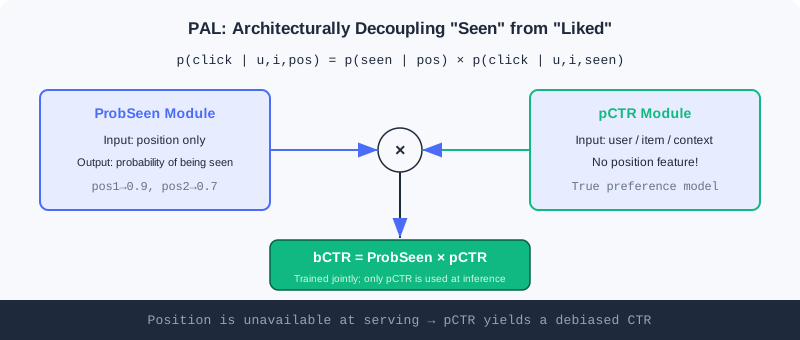
During offline training, the two module outputs multiply into the final CTR prediction:
The prediction is compared against the true label to compute the loss, and backpropagation optimizes both modules jointly.
The Train/Inference Separation Mechanism
PAL's core trick is to use different module combinations for training and inference:
- Training: the two modules are optimized jointly. The model automatically learns to assign credit — when a top item is clicked, part of the credit goes to the position effect (ProbSeen) and part to content quality (pCTR). This spares us from having to know each sample's "seen probability" in advance.
- Inference: only the pCTR module is used. Since it was designed during training to be position-free, it directly yields CTR predictions with position bias removed. You never need to assume a value for the position feature at inference.
💡 Key Insight: PAL is fundamentally information separation — position-related information is handled by ProbSeen, content-related information is preserved by pCTR; taking only the latter at inference naturally yields debiased preference. It neatly sidesteps the fundamental contradiction that "position is unavailable at inference time".
🧠 Mental Model: Separating "Bright Lights" From "Good Food"
Imagine a restaurant placing its signature dish under the brightest lamp (great position). You order it — maybe the dish is genuinely delicious, or maybe you just spotted it because the light was so bright. PAL's approach: one specialist records "the probability each lamp position gets noticed" (ProbSeen), while another purely judges "how good the dish itself is" (pCTR). The final score multiplies the two; but when you ask "is this dish actually good", you only ask the latter — the lamp's position no longer interferes.
Analysis: IPS and PAL represent two debiasing routes: generic data weighting (IPS, changes the loss) vs dedicated structural design (PAL, changes the architecture). IPS is flexible but plagued by variance and indirect for position bias; PAL handles position precisely with an elegant train/inference separation, but decouples only a single bias source. In practice they stack — first IPS compensates observation bias, then PAL handles position. Either way, the prerequisite is to understand how the bias arises rather than blindly fitting.
⚠️ Common Mistakes in 5.1
| # | Mistake | Example | Why It's Wrong | Fix |
|---|---|---|---|---|
| 1 | Treating "no interaction" as "negative" | A long-tail item with no clicks is labeled 0 and trained on directly | No interaction may mean no exposure (a potential positive); naive negative labeling injects exposure bias | Correct observation probabilities with IPS/an exposure model |
| 2 | Believing more extreme IPS is better | Not clipping weights; samples with tiny propensities get thousand-fold weights | Variance explodes and training diverges | Clip/normalize weights; balance unbiasedness against low variance |
| 3 | Treating PAL's pCTR as an ordinary CTR model | Feeding the position feature into pCTR at inference | pCTR is designed to be position-free; adding position reintroduces position bias | Use only pCTR at inference; leave position to ProbSeen |
| 4 | Ignoring the feedback loop | Debiasing once and calling it done | The loop keeps amplifying residual bias; a one-shot fix is not enough | Debias continuously across stages (data + model); monitor the Matthew effect |
| 5 | Mixing up the two bias fixes | Using IPS to handle position bias | IPS compensates unequal observation and doesn't fit structured position bias | Prefer PAL to decouple position bias |
Chapter Summary
📌 Key Takeaways
| Concept | Key Points | Why It Matters |
|---|---|---|
| Data bias | Selection/exposure/conformity/position, arising at collection | The root of all result bias; use the right tool |
| Result bias | Popularity/unfairness, amplified by the model | Directly harms personalization and fairness |
| Feedback loop | Recommend → interact → retrain, feeding each other | Left uncut, bias snowballs |
| IPS | , unbiased but high-variance | Generic debiasing; needs clipping for stability |
| PAL | Factorizes | Structurally decouples position from preference; inference uses pCTR only |
❓ FAQ
Q1: Since the data is biased, why not just collect unbiased data?
A: Production systems cannot randomize exposure the way lab experiments do (it would badly hurt user experience and metrics). You must debias on the biased observed data you have — IPS/PAL are designed exactly for this constrained setting.
Q2: IPS or PAL — which one?
A: If the bias comes from unequal observation probability (selection/exposure), prefer IPS; if it is a structured position effect, prefer PAL. They also stack, each targeting a different bias source.
Q3: Why does PAL jointly optimize both modules during training?
A: Nobody knows each sample's true "seen probability" and "post-seen click probability" in advance. Joint training lets the model learn to divide responsibility between the two itself, without manually labeled position tags.
Connections to Later Chapters
- 5.2 (cold start): bias and cold start often compound — new items get little exposure and are easily drowned by popularity bias; debiasing and cold start must work in concert.
- 5.3 (the generative paradigm): end-to-end generation optimizes a single model jointly, naturally weakening the inconsistent-objective bias introduced by cascaded architectures.
- Part 3 Ranking (Ch3.x): the scoring function is where IPS/PAL act most directly — debiasing usually lands in the loss or the CTR module.
Practice Problems
Work through all problems in order — they get progressively harder. Each has a complete solution you can reveal after trying it yourself.
Problem 5.1.1 — Bias Classification 🟢 Easy
Which of the four data biases (selection/exposure/conformity/position) does each scenario below belong to?
- (a) Users star-rate only videos they like and never flag the bad ones.
- (b) A newly launched niche documentary is almost never recommended and naturally gets few plays.
- (c) A product has tens of thousands of positive reviews, and a user follows the crowd with 5 stars.
- (d) Mediocre content in slot 1 gets 3× the CTR of quality content in slot 8.
💡 Solution (click to reveal)
Approach: Match each scenario against the four data-bias definitions: does the bias come from user habits, system exposure, group psychology, or list position?
- (a) Selection bias (MNAR): users rate only what interests them; neutral/negative ratings go unrecorded.
- (b) Exposure bias: the lack of plays may come from never being shown (a potential positive), not genuine disinterest.
- (c) Conformity bias: the rating is influenced by crowd opinion, not an independent true preference.
- (d) Position bias: clicks are strongly driven by rank position, independent of content relevance.
Key points:
- First ask which stage the bias arises in, then classify.
- (b) differs from popularity bias: popularity is the result; exposure is a cause at the data-collection stage.
Problem 5.1.2 — Computing IPS Weights 🟢 Easy
A user–item pair has observation probability . Write its IPS weight , and explain what happens if the naive method treats it as an ordinary sample (weight 1).
💡 Solution (click to reveal)
Approach: Apply the IPS weight formula directly.
This sample gets a 5× weight. Under the naive method with weight 1, this "rarely observed interaction" contributes only a single share, underweighting the strong preference signal it carries — especially when most samples have close to 1, the true information in this rare sample is almost drowned out.
Key points:
- Low propensity → high weight (inverse weighting).
- IPS's goal is not "treating every sample equally" but "recovering the true distribution according to how hard each sample was to observe".
Problem 5.1.3 — Explaining Why Unbiasedness Holds 🟡 Medium
What is the core idea behind proving ? Why does the naive estimator fail to achieve it? And why do production environments usually still clip IPS weights?
💡 Solution (click to reveal)
Approach: Understand it from the angle of "expectations correcting the observation distribution".
Why unbiasedness holds: the distribution of observed data is distorted by observation probabilities . IPS's weights discount over-sampled samples and boost under-sampled ones, realigning the weighted empirical distribution with the true distribution. In expectation, then equals the true risk over all pairs.
Why the naive estimator fails: averages directly over the distorted observation distribution, implicitly weighting by itself, so its expectation inherently deviates from .
Why clip: when some is tiny (e.g. 0.01), the reciprocal reaches 100 and a single sample can violently skew the gradient — the estimate's variance explodes and training destabilizes. Clipping (e.g. ) or normalization trades between "unbiased" and "low-variance"; it is an engineering necessity of the bias-variance tradeoff.
Key points:
- IPS uses reciprocal weights to "un-distort" the observation distribution → expectation aligns with the true distribution.
- Theoretically unbiased ≠ stable in practice; clip to control variance.
Problem 5.1.4 — Designing a PAL Retrofit 🔴 Hard
The ranking model you own uses a DeepFM to predict CTR, with "display position" as one of its training features. After launch you find that low-quality content near the top has overestimated CTR. Explain how to retrofit it with the PAL approach, specifying which modules training and inference each use and where the position feature goes.
💡 Solution (click to reveal)
Approach: Follow PAL's three steps: factorize + two modules + train/inference separation.
- Factorize: decompose the existing CTR into .
- Two modules: add a lightweight ProbSeen module that takes only position and outputs the "seen probability"; convert the original DeepFM into the pCTR module, removing its position features and keeping only user/item/context. During training the two outputs multiply into before the loss.
- Separate:
- Training: jointly optimize ProbSeen and pCTR, letting the model learn the responsibility split itself.
- Inference: use pCTR only (position-free). Position features never enter pCTR, and no position value needs to be assumed — pCTR directly outputs debiased CTR. Position information is used only by ProbSeen during training.
Now low-quality content near the top is no longer overestimated just because "the lamp is bright" — its pCTR reflects only the content's true appeal.
Key points:
- Strip the position feature out of pCTR and hand it to ProbSeen.
- Using pCTR alone at inference is how PAL solves "position being unavailable at inference time".
🏆 Challenge: Attack and Defense Under Compounding Biases
Suppose a short-video app where new creators' content (long-tail) gets minimal exposure, and the system ranks high-heat content first by default. Write an analysis of at most 200 words explaining how the feedback loop simultaneously amplifies popularity bias and position bias here, and give at least two stackable debiasing measures and which bias each targets.
💡 Hint
Loop logic: high-heat content ranks first → more clicks → more training samples → the model pushes high-heat content even more → long-tail gets even less exposure. Popularity bias is amplified by the skewed interaction distribution and can be compensated with IPS (weighting by exposure/observation probability); position bias is introduced by rank placement and can be handled with PAL decoupling the position effect from pCTR. Stacked, the two strike different bias sources; monitor the Matthew effect at the same time so a single measure is not cancelled out by the loop.
Cold Start
📝 Before You Continue: Make sure you have read collaborative filtering and the two-tower model in Part 2 Retrieval, and the bias perspective in 5.1. Cold start is, at its core, a bias predicament: being asked to be accurate with no history.
A recommender system's most awkward moment is when a new item goes on shelf, or a new user signs up. Collaborative filtering learns preferences from user–item interactions, but at that moment the interactions are zero; content-based methods can handle new items, but often capture only surface similarity.
This is the cold-start problem — the system's core engine (behavioral data) has not fired up yet, but it must immediately output trustworthy recommendations. This chapter splits cold start into two faces: content cold start (new items lack interactions) and user cold start (new users lack history), with two representative solutions for each. Their shared wisdom is borrowing strength: a new item borrows from content, a new user borrows from meta-knowledge or population structure.
After reading this chapter, you will be able to:
- Distinguish the fundamental difference between content cold start and user cold start
- Explain how CB2CF maps content features to collaborative-filtering representations so new items get CF quality directly
- Write down MetaEmbedding's two-stage meta-loss and understand that it optimizes "learnability" rather than a fixed vector
- Explain MeLU's parameter separation and POSO's "personalization submergence" insight, and compare the two
- Work through 4 tiered practice problems to consolidate the engineering and math intuition for cold start
5.2.0 The Two Faces of Cold Start
Cold start is not one problem but two objects each "lacking history":
| Type | What's Missing | Typical Failure | Solution Intuition |
|---|---|---|---|
| 🎬 Content cold start | New items lack user interactions | Collaborative filtering cannot compute similarity for them | Borrow content: map attributes onto existing representations |
| 👤 User cold start | New users lack behavior history | Can only recommend popular items, no personalization | Borrow meta-knowledge/populations: fast adaptation or segmentation |
We take each in turn.
5.2.1 Content Cold Start: Letting New Items "Borrow" Collaborative Quality
Collaborative filtering uncovers complex implicit associations but is helpless with new items; content-based methods handle new items but often capture only surface similarity. The ideal is: new items also get collaborative-filtering-grade representations — exactly the goal of CB2CF and MetaEmbedding.
CB2CF: From Content Features to Collaborative Representations
The core idea of CB2CF (Content-Based to Collaborative Filtering) is to learn a mapping function that maps an item's content features directly into the collaborative-filtering embedding space, yielding .
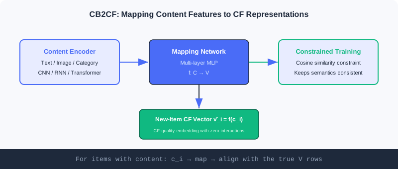
For items that have both a content description and rich interactions, we hold both their content vector and their CF embedding. CB2CF uses a deep network to learn the nonlinear mapping between the two representations, so a new item obtains a semantically consistent CF representation from content alone. Its multi-view architecture has three modules:
- Content Encoder: encodes multimodal content (text, images, categories) into a unified content vector. CNNs for images, RNN/Transformer for text.
- Mapping Network: the core — stacked fully-connected layers that learn the nonlinear map from content space to CF embedding space, capturing complex content–preference associations.
- Constraint Optimization module: uses a cosine-similarity constraint to keep the mapped representation semantically consistent with the true CF embedding, guaranteeing the mapping is valid.
Where do collaborative vectors come from? For items with interactions, CF vectors can be produced in several ways: matrix factorization , where item 's vector is row of , ; the item-tower output of a two-tower retrieval model; or deep methods like NCF and autoencoders. Once CB2CF has learned , a new item's content passes through to yield .
🧠 Mental Model: The Translator
Think of CB2CF as a translator. CF embeddings are the system's internal lingua franca; established items all speak it. A new item only speaks "content-ese" (text/images). The translator has learned to render content-ese into CF-ese, so even though the new item has never made friends (no interactions), the system understands it the moment it speaks and folds it into the collaborative network.
Analysis: CB2CF's strength is directness — one mapping and a new item instantly holds a CF-grade representation that plugs into existing retrieval/ranking. Its limits: the mapping's quality ceiling is bounded by how transferable "content → CF" is; if content correlates weakly with collaborative signal, the translation distorts. It also assumes existing items' CF vectors are trustworthy (you need a good CF model first).
MetaEmbedding: Meta-Learning "Smart" Initial Embeddings
CB2CF solves "new items can't get a CF representation", but another difficulty remains: even with an initial vector, traditional random initialization makes new items perform poorly early on and need lots of interactions to converge.
MetaEmbedding applies meta-learning to generate embeddings for new items that are both initially high-quality and quick to adapt. It optimizes the generator by simulating each item's full journey "from cold start to warmed up".
Algorithm inputs: a pretrained base model , an item set , meta-loss weight , and step sizes . For each sampled item :
Initial embedding generation stage: the generator produces the initial vector
where is item 's features and is the generator with parameters . Then sample two batches of samples each: and .
Gradient adaptation and evaluation stage: compute the loss on the first batch and take one gradient-adaptation step, simulating "after a few interactions":
Then evaluate the adapted loss on the second batch.
The key is the meta-loss balancing two objectives:
Finally, update the generator with the meta-losses of all sampled items:
💡 Key Insight: MetaEmbedding optimizes an embedding's "learnability", not the embedding itself. By repeatedly rehearsing "initialize → adapt → evaluate" on established items, it learns to give new items a "smart starting point" — one that converges to a high-quality representation after only a few real interactions.
🧠 Mental Model: Teaching "How to Learn" Instead of "Memorizing Answers"
MetaEmbedding is like a coach who doesn't hand a rookie the match answers, but trains him in "how to warm up before going on court and how to adjust through the first few plays". When the real match comes, he hits his stride after just a few real exchanges. weighs "is the opening stance good" against "how strong is he after fine-tuning".
5.2.2 User Cold Start: Fast Personalization for New Users
A newly registered user has no interaction history, so collaborative filtering can only serve generic popularity-based recommendations. User cold start focuses on: how to capture personalized preferences quickly from a few behaviors. MeLU and POSO offer two approaches — meta-learning and segmentation architecture.
MeLU: Learning Each User as a Separate Task
MeLU (Meta-Learned User preference estimator) treats each user's preference learning as an independent task, and uses MAML (Model-Agnostic Meta-Learning) to train a model that adapts quickly to new users. MAML's essence is "learning how to learn" — rather than being optimal on one task, it learns a good initialization such that a few samples suffice to adapt to a new task.
MeLU uses two tiers of parameters:
- governs the embedding parameters for users and items (shared by all users)
- holds the parameters of the model's core decision network (adapts quickly to each individual)
Training strictly follows MAML's two loops:
- Inner-loop adaptation: for each user , compute gradients from their interaction history and update locally: .
- Outer-loop meta-update: using all users' adapted parameters, update both sets of global parameters simultaneously:
MeLU's innovation is parameter separation: learns shared general representations while specializes in fast per-user adaptation. This retains representation capacity while personalizing quickly for new users. MeLU also proposes an evidence candidate selection strategy that picks the set of items most discriminative of user preferences for cold-start evaluation.
Analysis: MeLU's advantage is theoretical elegance — a new user gets personalized after a few gradient steps, no retraining from scratch. The costs: MAML's second-order gradients are computationally heavy, and it relies on the assumption that users' tasks are identically distributed; when new and old users' behavior distributions differ hugely, fast adaptation alone may not suffice.
POSO: Fighting "Personalization Submergence" with Segmented Submodules
POSO (Personalized cOld Start Modules) attacks from the architecture angle with a sharper insight: the root cause of user cold start is not just data scarcity, but the huge distributional gap between new and old users' behavior, plus the model's "submergence" when facing imbalanced distributions — when new users are far outnumbered by old ones, even with an "is new user" feature, training is dominated by the old-user majority. The model learns to ignore this heavily imbalanced feature, and the new users' personalization signal drowns.
POSO embeds into many module types; take the MLP as an example. The original MLP shares weights across all users, ; POSO introduces parallel submodules , plus a personalized gating network (taking such as is_new_user and activity level) that outputs weights . The final output is the weighted combination:
New users then rely mainly on "the submodule optimized for them" while old users use another set, effectively avoiding feature submergence. The idea extends to:
- POSO-MHA: extends to groups of attention heads, each with dedicated transforms, concatenated and aggregated within each group; gating selects group weights by user features.
- POSO-MMoE: shared experts at the bottom + expert groups at the top ( experts per group), stacking task gating and personalized gating for dual personalization at both the task level and the user-segment level.
🧠 Mental Model: Multiple Service Desks vs a Single Clerk
An ordinary model is like a single clerk serving all customers at once: biased toward the regulars' (old users') habitual requests, with newcomers' (new users') special needs drowned out. POSO is like opening dedicated desks: newcomers go to the "newcomer desk", regulars to the "regulars desk", and a greeter at the door (the gate) routes customers by type — newcomers' needs can never be shouted down by the regulars' volume.
Analysis: POSO and MeLU are complementary. MeLU assumes "all users are identically distributed; rely on fast adaptation" and suits scenarios with similar behavior patterns; POSO directly targets "imbalanced distributions causing feature submergence" and forces the split structurally — easier to integrate into off-the-shelf deep modules (MLP/MHA/MMoE) and free of meta-learning's heavy gradients. In practice they combine: use POSO's structure to keep cold start from being submerged, and meta-learning to further accelerate convergence.
⚠️ Common Mistakes in 5.2
| # | Mistake | Example | Why It's Wrong | Fix |
|---|---|---|---|---|
| 1 | Randomly initializing new-item embeddings | A new item enters the model with a random vector | Poor early performance; needs many interactions to converge | Use MetaEmbedding to generate a smart starting point |
| 2 | Mistaking content similarity for collaborative similarity | CB2CF relies only on text similarity | Surface similarity ≠ behavioral collaboration; the mapping distorts | Use constraint optimization to keep semantics consistent |
| 3 | Assuming MAML always beats structural design | Reaching for MeLU reflexively for user cold start | Insufficient adaptation when behavior distributions differ, plus heavy second-order gradients | Prefer POSO's structural split under imbalance |
| 4 | Assuming one new-user feature is enough | Adding only an is_new_user flag | Old users dominate training and the feature gets submerged | Use POSO submodules + gating to force the split |
Chapter Summary
📌 Key Takeaways
| Concept | Key Points | Why It Matters |
|---|---|---|
| Content cold start | New items lack interactions; CF fails | Borrow content mappings to obtain CF representations |
| CB2CF | , content→CF | New items gain collaborative quality instantly |
| MetaEmbedding | Two-stage meta-loss optimizing "learnability" | Generates initial vectors that adapt quickly |
| User cold start | New users lack history; only popular items can be recommended | Borrow meta-knowledge/population structure for fast personalization |
| MeLU / POSO | Meta-learned adaptation / segmented submodules against submergence | Two complementary user cold-start approaches |
❓ FAQ
Q1: Do CB2CF and MetaEmbedding solve the same problem?
A: Not quite. CB2CF solves "new items cannot obtain a CF representation"; MetaEmbedding solves "even with an initial vector, random initialization converges slowly". They can chain: MetaEmbedding generates a good starting point, then a CB2CF-style mapping supplies CF quality.
Q2: Why is POSO more effective than just adding an is_new_user feature?
A: Because training is dominated by old users, a lone feature gets "submerged" — the model learns to ignore it. POSO uses dedicated submodules plus gating to structurally force new users through their own pathway, which cannot be ignored.
Q3: How to choose between MeLU and POSO?
A: If user behavior patterns are similar and few samples suffice to adapt → MeLU; if new/old user distributions differ greatly and features are easily submerged → POSO. They can also be combined.
Connections to Later Chapters
- 5.1 (debiasing): long-tail new items get little exposure and are easily drowned by popularity bias; cold start and debiasing must work in concert.
- 5.3 (generative): semantic IDs let new items be recommended without any behavior, easing content cold start at the representation level.
- Part 2 Retrieval (Ch2.x): the CF representations produced by CB2CF plug directly into two-tower/vector retrieval.
Practice Problems
Work through all problems in order — they get progressively harder. Each has a complete solution you can reveal after trying it yourself.
Problem 5.2.1 — Distinguishing Cold-Start Types 🟢 Easy
Is each scenario below content cold start or user cold start?
- (a) A newly launched documentary with no play records needs to be retrieved.
- (b) A freshly registered user has tapped only 3 videos, yet the system keeps recommending popular content.
- (c) A newly released song should go straight into personalized playlists, not just the "New Releases" list.
💡 Solution (click to reveal)
Approach: Ask whether what's missing is item history or user history.
- (a) Content cold start: the item has no interactions; collaborative filtering fails.
- (b) User cold start: the user lacks history; only popular items can be recommended.
- (c) Content cold start: the new song (item) lacks behavior and wants to enter personalization by borrowing content.
Key points:
- The "subject" of content cold start is a new item; of user cold start, a new user.
- Their solutions differ: items borrow content mappings; users borrow meta-learning/segmentation.
Problem 5.2.2 — Filling In the CB2CF Mapping 🟢 Easy
CB2CF learns a mapping function that maps a new item's content features into the collaborative-filtering space. Complete the output expression and explain the role of the constraint optimization module.
💡 Solution (click to reveal)
Approach: Recall CB2CF's three modules and the mapping definition.
The mapping output is:
where is realized by the mapping network (stacked fully-connected layers). The constraint optimization module applies a cosine-similarity constraint to keep semantically consistent with the true CF embedding — otherwise the mapping might "appear to converge" while drifting away from the collaborative space, causing new items to be wrongly recommended.
Key points:
- A new item has no interactions, yet its content through yields a CF representation.
- Constraint optimization is what guarantees the mapping works; do not skip it.
Problem 5.2.3 — Interpreting the MetaEmbedding Meta-Loss 🟡 Medium
MetaEmbedding's meta-loss is . Explain: (1) what do the two terms each measure? (2) What happens if ? (3) Why is it said to optimize "learnability" rather than the embedding itself?
💡 Solution (click to reveal)
Approach: Decompose the meta-loss against the two-stage process.
(1) measures the initial embedding's direct quality on the first batch (cold-start opening performance); measures quality after one gradient-adaptation step (adaptation performance after a few interactions).
(2) If , only remains; the generator optimizes initial quality only and no longer cares about "can it adapt quickly" — new items get a good starting point but are hard to fine-tune, defeating the purpose of fast cold-start convergence.
(3) It does not fix a dead vector for a specific item; instead it repeatedly rehearses "initialize → adapt → evaluate" on many established items, learning to generate starting points with good initial performance and strong adaptation potential. Faced with a real new item, that starting point converges quickly with a little real data — what's optimized is "how learnable it is".
Key points:
- balances "opening" against "adaptation".
- Meta-learning = learning how to learn, not learning a fixed answer.
Problem 5.2.4 — Designing a POSO Retrofit 🔴 Hard
You have a weight-shared MLP ranking model. Online, recommendations for new users perform far worse than for old users, even though an is_new_user feature has been added. Propose a retrofit following the POSO-MLP approach: write out the mathematical form of the submodules and the gate, and explain why this solves "feature submergence".
💡 Solution (click to reveal)
Approach: Follow POSO-MLP's three-part retrofit.
Submodules: introduce parallel MLP submodules, each with independent weights:
Gate: the personalized gate takes (including is_new_user, activity level, etc.) and outputs per-submodule weights:
Final output: the weighted combination of all submodules:
Why it solves submergence: in the original model all users share , training is dominated by old users, and the lone is_new_user feature is easily learned to be "ignored". POSO routes new users mainly through "new-user-dedicated submodules" and old users through another set, structurally guaranteeing new users' personalization signal a dedicated pathway that the old users' volume cannot drown.
Key points:
- The key is "structural routing", not "adding features".
- The gate dynamically allocates submodule weights by user features, smoothly transitioning between new and old users.
🏆 Challenge: A Cold-Start Combo
A short-video app faces both at once: new creators' content (content cold start) and newly registered users (user cold start). Write a plan of at most 200 words explaining how you would combine CB2CF / MetaEmbedding / POSO to address each, and identify which step depends most on "the quality of existing items' CF vectors".
💡 Hint
- New creators' content: use MetaEmbedding to generate a smart initial embedding, then borrow a CB2CF-style content→CF mapping to obtain a collaborative representation and plug into retrieval.
- Newly registered users: use POSO submodules + gating for structural routing so
is_new_userisn't submerged; with a few behaviors available, stack MeLU-style fast adaptation on top. - The step most dependent on "existing items' CF vector quality" is CB2CF — its constraint optimization needs trustworthy true CF embeddings as alignment targets; if the underlying CF model is poor, the mapping distorts too.
Evolution of the Generative Paradigm
📝 Before You Continue: Make sure you have read the two paradigms and the four capability-evolution stages in 1.1, and the semantic/cold-start foundations in 5.2. This chapter is the "hands-on edition" of Part 1's two paradigms — turning abstract concepts into concrete models.
In 1.1 we planted a thread: recommendation can shift from "discriminative scoring" to "generative sequence generation", much like understanding and producing natural language as a special kind of "language". The earlier chapters of this part followed the discriminative three-stage pipeline through industrial practice; now it is time to return to that thread and see how the generative paradigm concretely evolves.
At its core is a redesign of three elements: how the input is organized (from item-ID sequences to heterogeneous event streams), what the output generates (from atomic IDs to semantic representations), and how objectives and architecture trade off (expressiveness vs computational efficiency). Along these three questions, generative recommendation has taken three clear paths — generative retrieval, generative ranking, and end-to-end unified generation.
After reading this chapter, you will be able to:
- Connect the capability leap of "memorization · generalization → understanding · reasoning" against Part 1's two paradigms
- Explain how HSTU unifies heterogeneous information into event streams and how TIGER reshapes the output with semantic IDs
- Distinguish generative ranking (GenRank / MTGR) from discriminative ranking in essence
- Describe OneRec's four key innovations in end-to-end generation, especially iterative preference alignment (IPA)
- Work through 4 tiered practice problems to consolidate the mapping from paradigm to model
5.3.0 From "Selecting the Best" to "Creating": A Paradigm Shift
Looking back at Part 1's two storylines: the discriminative approach asks "will the user like this candidate?" — selection; the generative approach asks "what does the user want to see next?" — creation. Generative retrieval (e.g. SASRec) has already validated that treating the user's behavior sequence as "language" and autoregressively predicting the next item is feasible.
But the real change goes beyond "swapping in a generative objective" — it systematically reshapes the input, the output, and the architecture. The table below contrasts each path's focus:
| Path | Element Reshaped | Representative Models |
|---|---|---|
| Generative retrieval | Unified input + semantic output | HSTU, TIGER |
| Generative ranking | Autoregression brought into the ranking stage | GenRank, MTGR |
| End-to-end unified generation | A single model replaces the full pipeline from retrieval to ranking | OneRec |
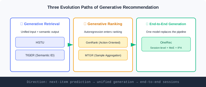
💡 Key Insight: These three paths do not replace one another; they are progressively cumulative — first prove generation works for retrieval, then push generative thinking into ranking, and finally let one model swallow the entire pipeline. Each step answers one of the questions "input / output / architecture".
5.3.1 Deepening Generative Retrieval: Redoing the Input and the Output
Generative retrieval deepens beyond SASRec in two directions: HSTU deepens the understanding of the "input", while TIGER fundamentally reshapes the definition of the "output".
HSTU: Unifying Everything into Event Streams
HSTU is no longer content with plain item-ID sequences; it uniformly encodes all of a user's heterogeneous information — attributes, behavior types, timestamps — into one rich "event stream". It learns the conditional distribution , where is the user's comprehensive representation at the current moment and is the next candidate item.
Two technical innovations are especially key:
- Unified feature handling: categorical features are flattened by timestamp into a unified sequence, e.g.
[(feature:age,value:30), (action:login), (action:view,item:A)]; numerical features are modeled implicitly so the model infers them itself. - Point-wise aggregation: it abandons the traditional Transformer's softmax normalization in favor of point-wise aggregation . The motivation: in recommendation, the "intensity" of user interest is a key signal, but softmax forcibly normalizes all historical attention weights, distorting true preference intensity.
By switching the prediction target and training head, HSTU can also operate as a ranking rather than retrieval task — a testament to the flexibility of generative architectures.
🧠 Mental Model: From a "Ledger of Records" to an "Event Stream"
The discriminative approach treats user history as a "list of candidate items" to score one by one; HSTU treats it as a timestamped, action-typed, context-rich "diary of life". Instead of splitting "viewed A", "logged in", and "age 30" apart, it strings them into a chain of events over time, so the model reads the full information of both "intensity" and "order" — like reading a friend's diary rather than only their receipts, you know them far better.
TIGER: Reshaping the Output with "Semantic IDs"
TIGER argues that predicting semantics-free atomic IDs is inefficient and hurts generalization, and instead generates structured "semantic IDs" to represent items. The pipeline has two stages:
Stage 1 — generating semantic IDs: use a Residual-Quantized Variational AutoEncoder (RQ-VAE). For an item's content feature vector , the encoder maps it to a latent representation ; then quantization layers each find, at layer , the codeword in the codebook closest to the current residual :
The result is a semantic-ID tuple .
Stage 2 — sequence-to-sequence generation: the user's historical interactions are converted into the corresponding semantic-ID sequence, and an Encoder-Decoder Transformer is trained to autoregressively generate the next item's semantic ID. The advantages:
- Semantic sharing: items with similar content have similar semantic IDs, enabling knowledge sharing;
- Cold-start advantage: semantic IDs can be generated for brand-new items and recommended directly (echoing content cold start in 5.2);
- Structured representation: multi-layer codewords represent large item corpora efficiently.
The costs: it may generate invalid IDs, and inference is expensive — a trade-off between expressiveness and computational efficiency.
Analysis: HSTU and TIGER tackle the "input" and the "output" respectively, matching Part 1's capability evolution from "generalization" (deeply understanding heterogeneous signals) to "understanding" (items encoded as semantics-carrying tokens). TIGER's semantic IDs are a natural antidote to cold start — new items are understood without any accumulated behavior. Yet both remain "retrieval-layer" generation and have not yet shaken ranking and re-ranking.
5.3.2 Generative Ranking: Pushing Autoregression into the Ranking Stage
Generative ranking brings autoregressive thinking into the traditional ranking stage, along two main technical routes.
GenRank: Action-Oriented Sequence Organization
GenRank adopts an "action-oriented" design, redefining ranking as predicting the user's action probability for a given candidate, . The core insight: predicting behavioral actions (click, like) is computationally cheaper than predicting the next item ID — the action space is far smaller than the item space.
Architecturally, GenRank treats items as known positional context and focuses on predicting the action at each position; the input is the sum of five embeddings (item, action — candidates use a special [MASK] embedding, position, request index, time). It replaces learnable relative attention bias with ALiBi (attention with linear biases) — a parameter-free static penalty that cuts attention computation cost by roughly 75% and speeds up training by 94.8%.
MTGR: Per-User Sample Aggregation
MTGR tries to retain a traditional DLRM's rich features while gaining the scalability of a generative architecture. Its core innovation is per-user sample aggregation: all candidates of a user are aggregated into a single sample [user_features, [candidate_1_features, ..., candidate_K_features]], so user-related features are computed once and shared across all candidates.
To process such heterogeneous sequences, MTGR introduces Group Layer Normalization (GLN) — normalizing tokens from different semantic spaces (user profile, item features) separately — and a dynamic masking strategy — static user features are visible to all tokens, dynamic user features follow causality, and candidate tokens cannot see each other to prevent information leakage.
⚠️ Warning: Despite the "generative" label, MTGR is essentially a ranking model — its "generative" aspect is mainly architectural style (processing token sequences with a Transformer); the final goal remains discriminative scoring and ranking. Don't be misled by the name: it is discriminative dressed in generative clothing.
🧠 Mental Model: The Judge Reads the Entries Differently
In discriminative ranking, the "judge" flips through each contestant's resume and scores it. GenRank/MTGR change the judge's way of reading — spreading all candidates side by side and scanning them at once with attention (the compute advantage of generative architectures). But the judge still ends up scoring and selecting, and has not become the friend who "writes out the list directly". That is the fundamental divide between generative ranking and end-to-end generation.
5.3.3 End-to-End Unified Generation: OneRec's Highest Form
OneRec represents the highest form of generative recommendation — end-to-end unified generation, where a single model runs the entire pipeline from retrieval to ranking. Its core innovation is session-level generation: instead of predicting a single next item, it directly generates an ordered recommendation list (typically 5–10 items), defined as a "session".
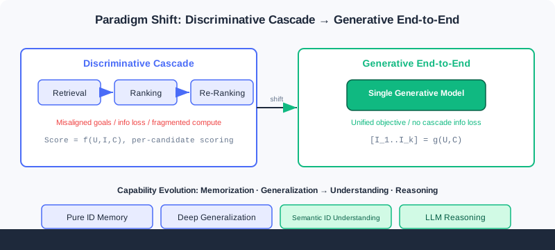
OneRec uses a standard Encoder-Decoder with three important extensions:
- Semantic item representation: multi-level vector quantization turns each item into a sequence of semantic tokens, so the model understands content meaning rather than bare IDs.
- Sparse Mixture-of-Experts (MoE): MoE layers in the decoder's feed-forward networks activate a few expert subnetworks, significantly increasing capacity without a proportional increase in compute.
- Iterative Preference Alignment (IPA): the most innovative component, addressing the difficulty of obtaining explicit preference-comparison data in recommendation.
The IPA mechanism: first train a reward model to predict session quality (watch time, likes, etc.); use the current OneRec to generate multiple candidate sessions for a sample (usually 128); score them with the reward model, taking the highest-scoring as the "chosen" response and the lowest-scoring as the "rejected" response ; finally update the model with a DPO (Direct Preference Optimization) loss.
Deployed online, OneRec delivered a 1.68% increase in total user watch time, proving the practical value of end-to-end unified generation. The cost is training complexity: the quantization model, the base generative model, and the reward model must be trained in sequence, followed by an iterative IPA-DPO loop — demanding on engineering.
🧠 Mental Model: From "Screening Resumes in Rounds" to "Writing the List in One Go"
The discriminative cascade is like hiring via HR: a massive open call first (retrieval), then ranked interviews (ranking), then final headcount decisions (re-ranking) — three teams each owning one stage, with information lost in handoffs and objectives pulling apart. OneRec is like a manager who knows the business and holds the authority, writing out the complete hire list in one go (session-level generation) — done in a single stroke, with one unified objective. This is what Part 1 calls "end-to-end dissolving the three pains of the cascade".
Analysis: End-to-end generation gains unified optimization, no cascade information loss, and concentrated compute; its costs are steeply higher training complexity and inference overhead, plus the supporting cast of DPO/reward models. It is no free lunch — complexity moves from "multi-stage coordination" to "single-model training engineering". Echoing Part 1: the generative approach replaces the discriminative "selection" with "creation", pushing memorization · generalization all the way to understanding · reasoning.
The interactive demo below visually contrasts the "discriminative cascade" with "generative end-to-end":
Click "Next" or "Autoplay" to watch the three-stage cascade being replaced by a single generative model, and see how the paradigm shift maps to the "understanding · reasoning" stage of capability evolution.
⚠️ Common Mistakes in 5.3
| # | Mistake | Example | Why It's Wrong | Fix |
|---|---|---|---|---|
| 1 | Taking MTGR as truly generative | "MTGR generates recommendations end to end" | It still ends in discriminative scoring; only the architectural style is generative | Recognize the real objective: generative ranking ≠ end-to-end generation |
| 2 | Assuming semantic IDs always beat atomic IDs | Replacing all retrieval with TIGER reflexively | Semantic IDs can generate invalid tokens and are pricier at inference | Weigh expressiveness vs efficiency; hybridize when needed |
| 3 | Confusing HSTU's input and output innovations | "HSTU uses semantic IDs for its output" | HSTU works on input unification; semantic IDs belong to TIGER | Keep them straight: HSTU = input, TIGER = output |
| 4 | Ignoring OneRec's engineering cost | Copying end-to-end without the DPO stack | Without a reward model/IPA, training cannot align preferences | End-to-end needs the full chain: quantization + generation + reward + DPO |
Chapter Summary
📌 Key Takeaways
| Concept | Key Points | Why It Matters |
|---|---|---|
| HSTU | Heterogeneous information unified into event streams + point-wise aggregation preserving intensity | Generative retrieval's deepening of the "input" |
| TIGER | RQ-VAE generates semantic IDs; autoregressive generation | A fundamental reshaping of the "output"; a natural cold-start fix |
| GenRank / MTGR | Action-oriented / sample aggregation | Generative thinking enters ranking; MTGR stays discriminative |
| OneRec | Session-level + MoE + IPA (DPO) | End-to-end unified generation swallowing the whole pipeline |
| Paradigm shift | Discriminative selection → generative creation | Maps to capability evolution: understanding · reasoning |
❓ FAQ
Q1: What separates generative retrieval (HSTU/TIGER) from end-to-end generation (OneRec)?
A: The former only replaces per-candidate scoring with candidate generation at the "retrieval" layer; the latter uses one model to directly generate the entire session list, swallowing the full pipeline from retrieval to ranking. The span goes from "point prediction" to "unified generation".
Q2: Why does TIGER ease cold start?
A: Semantic IDs are generated from content features (RQ-VAE), so new items obtain structured tokens without any accumulated behavior and can be generated into recommendations — exactly the "borrowing content" that content cold start in 5.2 calls for.
Q3: Why does OneRec's IPA use DPO instead of direct supervision?
A: Recommendation rarely has "explicit preference-comparison data". IPA uses the reward model to pick the highest/lowest scorers among 128 candidates as "chosen/rejected" pairs, then aligns with DPO — bypassing the lack of annotations.
Connections to Later Chapters
- 1.1 / 1.2 (paradigms and the map): this chapter grounds those two threads at the model level: discriminative → generative, and memorization · generalization → understanding · reasoning.
- 5.2 (cold start): TIGER's semantic IDs and CB2CF reach the same destination by different routes — both let new items be understood by borrowing content.
- The follow-up volume (Ch6–Ch10) builds on this chapter's OneRec to cover Scaling Laws (HSTU architecture), reasoning recommenders (OneRec-Think), diffusion models, and more.
Practice Problems
Work through all problems in order — they get progressively harder. Each has a complete solution you can reveal after trying it yourself.
Problem 5.3.1 — Classifying Generative Models 🟢 Easy
Assign each model below to one of the three evolutionary paths (generative retrieval / generative ranking / end-to-end generation):
- (a) HSTU (b) OneRec (c) GenRank (d) TIGER (e) MTGR
💡 Solution (click to reveal)
Approach: Match each path's focus element and representative models.
- (a) HSTU → generative retrieval (reshapes the input: event streams)
- (d) TIGER → generative retrieval (reshapes the output: semantic IDs)
- (c) GenRank → generative ranking (action-oriented)
- (e) MTGR → generative ranking (per-user sample aggregation, but discriminative at heart)
- (b) OneRec → end-to-end generation (a single model swallows the full pipeline)
Key points:
- HSTU/TIGER sit at the retrieval layer; GenRank/MTGR at the ranking layer; OneRec spans the full pipeline.
- Though called generative, MTGR's objective remains discriminative scoring.
Problem 5.3.2 — Computing TIGER Semantic IDs 🟢 Easy
Given an item content feature , the RQ-VAE encodes it to , with the first-layer residual . In the codebook , the codeword closest to has index , corresponding to . Write the selection formula for and the expression updating the residual .
💡 Solution (click to reveal)
Approach: Apply TIGER's quantization formulas directly.
Codeword selection:
So .
Residual update:
Key points:
- Each layer finds the nearest codeword in the codebook, then subtracts it from the residual.
- Iterating over layers yields the semantic-ID tuple .
Problem 5.3.3 — Telling "True" From "Fake" Generative 🟡 Medium
Someone claims: "MTGR processes token sequences with a Transformer, so it is end-to-end generative recommendation." Point out what is wrong, and explain the key difference between GenRank and OneRec regarding "truly generative or not".
💡 Solution (click to reveal)
Approach: Judge generativeness by the "final objective", not the "architectural style".
The error: although MTGR uses Transformer/attention (generative architectural style), its final objective is still discriminative scoring for ranking — the candidates are known and scored one by one. It is merely "discriminative in generative clothing", not end-to-end generation.
GenRank vs OneRec: GenRank is still generative ranking — it autoregressively models action probabilities, but the candidate set is known, the outputs are actions/scores, and retrieval and re-ranking remain untouched. OneRec is the real end-to-end generation — a single model directly generates an ordered session list (5–10 items), replacing the entire pipeline from retrieval to ranking, with the objective shifting from "scoring" to "creating sequences".
Key points:
- The criterion is "the objective: score-and-select or create sequences", not "whether a Transformer is used".
- Generative ranking ≠ end-to-end generation; the gap is an order of magnitude.
Problem 5.3.4 — Designing OneRec's Alignment Pipeline 🔴 Hard
You are to run preference alignment on OneRec. Write out the complete IPA steps (including the number of candidates and the definitions of chosen/rejected responses), explain why DPO rather than direct supervision, and identify the three prerequisite models the pipeline depends on.
💡 Solution (click to reveal)
Approach: Unfold the IPA mechanism step by step.
Steps:
- Train a reward model to predict session quality (watch time, likes, etc.).
- Use the current OneRec to generate 128 candidate sessions for a training sample.
- The reward model scores all candidates; the highest score becomes the "chosen" response , the lowest the "rejected" response .
- Update OneRec's parameters with the DPO loss.
Why DPO rather than direct supervision: recommendation rarely has "explicit preference-comparison data" (users won't label "which of these two lists is better"). IPA uses the reward model to construct "chosen/rejected" pairs from the model's own generated candidates, bypassing the annotation shortage; DPO needs no separate critic and optimizes the policy directly on such comparison pairs — stable and efficient.
Three prerequisite models: (1) the semantic representation model with multi-level vector quantization (item → tokens); (2) OneRec's base generative model; (3) the reward model. All three must be in place before the IPA-DPO loop can run.
Key points:
- IPA = self-generated candidates → reward scoring → chosen/rejected pairs → DPO.
- DPO removes the core obstacle of "no explicit preference annotations".
- End-to-end engineering is costly: the full chain of quantization + generation + reward + DPO.
🏆 Challenge: Arguing a Paradigm Migration
Suppose your company runs a discriminative three-stage system (retrieval + ranking + re-ranking) whose metrics have hit a plateau. Write an argument of at most 200 words: which signals should prompt you to try "generative ranking (e.g. GenRank)" first rather than jumping straight to "end-to-end generation (OneRec)"? Also state the risks and benefits of this incremental path.
💡 Hint
Signals favoring generative ranking first: the ranking stage suffers severe compute fragmentation and high attention cost (GenRank's ALiBi cuts compute by 75%), while mature retrieval/re-ranking stages are best left untouched. The benefits of the incremental path: controlled risk, quick local wins, no wholesale rewrite; the risks: still constrained by cascade information loss and misaligned objectives — the root cause remains. Once ranking validates the generative value and engineering is ready with quantization + reward + DPO, move up to OneRec for end-to-end. This echoes Part 1's "three pains of the cascade" and the progressive logic of this chapter's three paths.
Generative recommendation is shifting recommender systems from the discriminative paradigm of "scoring and ranking a candidate set" to the generative paradigm of "directly generating recommendation results." This is more than an upgrade in model architecture — it is a fundamental rethinking of the modeling philosophy. As the starting point of the "generative recommendation mainline," this part systematically builds four pillars: from paradigm motivation (why generative is needed), to architectural foundations (which models implement generation), then to the LLM modeling pipeline (how to train such models), and finally to Tokenizer technology (how recommendation data adapts to the interfaces of generative models). The four pillars build on one another, together forming the complete foundation you need for the later chapters — from scaling architectures to end-to-end generation, from thinking recommenders to diffusion models.
What This Part Covers
| Section | Topic | The Big Idea |
|---|---|---|
| 6.1 | Introduction to the Generative Recommendation Paradigm | Discriminative vs. generative: local scoring decisions vs. global probability modeling; three inherent limitations driving the paradigm shift |
| 6.2 | Foundations of Generative Architectures | Transformer self-attention / positional encoding / two architectural paradigms / causal masking, complemented by Diffusion |
| 6.3 | LLM Foundations | The pretraining–instruction tuning–preference alignment three-stage paradigm, and its mapping and challenges for generative recommendation |
| 6.4 | Codebook Quantization and Semantic IDs | Sparse ID / text / semantic ID paradigms; VQ-VAE, RQ-VAE, RQ-Kmeans, and RQ-OPQ industrial solutions |
What You'll Be Able to Do After This Part
- 🟢 Distinguish the core formulas and "questions asked" of discriminative vs. generative models, and list the three inherent limitations of the discriminative paradigm
- 🟢 Explain the Q/K/V mechanism of self-attention, positional encoding (including time-aware variants), and the role of causal masking
- 🟡 Compare the strengths, weaknesses, and applicable scenarios of Encoder-Decoder vs. Decoder-Only architectures
- 🟡 Restate the three-stage LLM paradigm (pretraining / SFT / RLHF / DPO) and map it to recommendation scenarios
- 🔴 Derive the three VQ-VAE losses and RQ-VAE residual quantization, and explain the three key values of semantic IDs
- 🔴 Complete 18+ tiered practice problems across 4 chapters, consolidating the full chain from paradigm to semantic ID
Core Concepts
| Concept | Section | Relevance |
|---|---|---|
| Discriminative / generative paradigms | 6.1 | The master switch of the book's generative mainline |
| Self-attention / positional encoding / causal masking | 6.2 | Core mechanisms of Transformer generative architectures |
| Encoder-Decoder vs. Decoder-Only | 6.2 | The fundamental trade-off in generative architecture selection |
| Diffusion models | 6.2 | A generation mechanism complementary to Transformer |
| Pretraining / SFT / RLHF / DPO | 6.3 | The methodological framework of LLM training paradigms |
| Item tokenization / semantic IDs | 6.4 | The bridge connecting recommendation data to generative models |
| VQ-VAE / RQ-VAE / RQ-Kmeans / RQ-OPQ | 6.4 | The technology spectrum for discretizing semantic IDs |
Prerequisites
- You have finished Part 1 (the two paradigms in 1.1, the technology map in 1.2)
- You have finished Part 2 (the inner product and vector-space intuition of the two-tower model in 2.3)
- Basic linear algebra (matrices, inner products), probability (softmax, KL divergence), and general neural network knowledge
This part covers frontier material with recent terminology (generative retrieval, semantic IDs, RQ-VAE, Scaling Laws, etc.). Every term is given in both Chinese and English on first appearance, with mental models and diagrams.
Tips for This Part
- Look at the motivation before the technology. The "why generative" discussion in 6.1 is the key to everything that follows — each technology responds to a specific discriminative limitation.
- Grasp the "unified architecture" mainline. From the Transformer in 6.2, to the LLM in 6.3, to semantic IDs in 6.4, "unified, scalable, end-to-end" is the design philosophy throughout.
- Get hands-on with the visualizations. The interactive HTML and SVG demos in each chapter are worth walking through yourself, grounding abstract formulas in intuition about "how sequences are generated" and "how vectors are quantized."
- Think against the discriminative paradigm. Whenever you meet a generative component, first ask: "which discriminative limitation does it solve?"
Let's dive in! 🚀
Foundations of the Generative Recommendation Paradigm
📝 Before You Continue: Please read the "two fundamental paradigms" section of 1.1 and the discriminative retrieval/ranking in 2.x first. This chapter pushes the discriminative-vs-generative contrast from intuition into modeling philosophy and architecture, and it is the theoretical starting point for all later generative chapters.
Over the past decade, recommender systems have evolved from traditional machine learning to deep learning, with ever-stronger models and ever-better business metrics. Yet one fact is easy to overlook: no matter how the models changed, the underlying modeling paradigm never did — we have been doing "discrimination" all along.
Given a set of candidate items, a discriminative model judges whether the user will like each one — at its core, a classification or ranking problem. This framework is extremely mature in industry, but it has gradually exposed deep limitations: misaligned objectives from multi-stage cascades, the difficulty of capturing sequential dependencies when scoring each item independently, and embedding parameters too sparse to feed modern hardware.
It is against this backdrop that Generative Recommendation has emerged as a brand-new paradigm. It no longer treats recommendation as "scoring a candidate set," but redefines it as a sequence generation task — the model directly learns "which items the user will interact with next." This seemingly subtle shift brings fundamental changes: from local scoring decisions to global probability modeling, from multi-stage cascades to end-to-end optimization, from a fixed candidate set to an open generation space.
After reading this chapter, you will be able to:
- Write down the core conditional probability formulas of discriminative and generative models, and explain how the "questions they ask" differ
- List the inherent limitations of the discriminative paradigm in parameter efficiency, semantic modeling, and multi-stage cascades
- Explain how generative autoregressive modeling naturally captures sequential dependencies and opens the door to end-to-end optimization
- Compare the essential differences between the two paradigms along three dimensions: objective function, information flow, and model architecture
- Complete 4 tiered practice problems to consolidate the "discriminative vs. generative" modeling philosophy
6.1.0 Discriminative Recommendation: How We Have Always Done It
The core of discriminative recommendation is learning a conditional probability distribution that predicts the probability of a positive interaction (click, purchase, etc.) between user and item under context . This modeling approach is intuitive and efficient, and it is by far the dominant approach in industry.
Modern deep learning recommendation models almost all follow the "Embedding & MLP" paradigm: user IDs, item IDs, and various features are first mapped to dense vectors through embedding layers, then processed by MLPs or more sophisticated feature interaction modules, and finally a scalar score is produced indicating the strength of the user's interest in the item. It is highly flexible — different feature interaction modules (FM, DeepFM, DCN, etc.) capture high-order feature crossing, while sequence modeling modules (DIN, SIM, etc.) characterize short-term and long-term preferences.
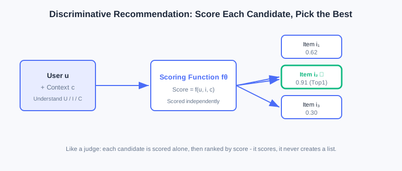
By integrating user features , item features , and context features , discriminative recommendation scores every candidate item one by one, predicting the probability of "a positive interaction occurring."
💡 Key Insight: The inputs of a discriminative model are exactly the same as a generative one (both must understand the user, items, and context), but the question it asks is "should this item be recommended" — a local, per-candidate binary classification problem.
Three Inherent Limitations of the Discriminative Paradigm
However, this "score each item independently" modeling approach also brings three problems that are hard to cure at the root.
① Parameter inefficiency. Embedding layers typically account for more than 90% of model parameters, yet these parameters are sparse and inefficient, hard to fully utilize on modern GPUs/TPUs. Huge numbers of parameters "sleep" in sparse ID lookup tables, and hardware utilization (MFU) stays persistently low.
② Missing semantic modeling. A discriminative model treats every item as an independent atomic unit. There is no semantic relationship between item IDs whatsoever. The IDs of two "sci-fi thrillers" have no prior connection in vector space; the model can only "memorize by brute force" their similarity from massive behavioral data, making the cold-start problem hard to solve.
③ The multi-stage cascade dilemma. To handle massive item catalogs and millisecond-level latency, industrial systems have to adopt a multi-stage cascade of "retrieval — coarse ranking — fine ranking — re-ranking." Each stage is handled by a different model with different optimization objectives (retrieval cares about relevance, ranking cares about CTR), so global objectives are hard to align; worse, every cascade stage loses information — high-quality items filtered out during retrieval by crude similarity computation never even get seen by later stages. This level-by-level filtering guarantees efficiency, but it traps the system in a "local optimum" and makes true end-to-end optimization impossible.
⚠️ Warning: These three limitations are not "engineering flaws" of discriminative models — they are intrinsic properties of the "per-candidate scoring" modeling paradigm. Curing them requires working on the paradigm itself, which is precisely the motivation for generative recommendation.
6.1.1 Generative Recommendation: Redefining the Task
Generative recommendation fundamentally redefines the recommendation task. Instead of treating recommendation as a discriminative problem of scoring a candidate set, it models recommendation as a sequence generation process. Given user , context , and the historical interaction sequence , generative recommendation learns the generation probability of this sequence:
This formula looks plain, but it hides a profound modeling idea: it no longer views each item in isolation, but treats the user's interaction behavior as a continuously evolving process. What the model learns is not "should a certain item be recommended," but "given the known history of behavior, which item is the user most likely to interact with next."
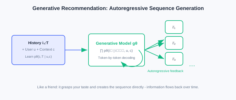
Conditioned on the user's historical interaction sequence, generative recommendation directly generates the next item (or the next segment of items) through autoregressive decoding — no need to evaluate candidates one by one.
🧠 Mental Model: Judge Scoring vs. Friend Recommending
Picture the two paradigms as two kinds of people. The discriminative model is like a talent-show judge: contestants (candidate items) fill the stage, the judge scores each one individually and hands out passes by score — it never "calls out the list directly," only scores. The generative model is like a friend who knows your taste well: without going through every option, they just say "you should watch these next," because they already understand the thread of your preferences. The former selects the best; the latter creates.
Why Autoregressive Modeling Is the Watershed
The advantage of autoregressive modeling goes beyond capturing sequential dependencies — it opens the door to end-to-end optimization:
- Eliminating error accumulation: the model generates recommendation results in a single forward pass, without depending on a multi-stage cascade, thus eliminating cascade-induced error accumulation and objective misalignment.
- Supporting global objectives: a generative model can optimize global objectives (such as long-term user satisfaction, platform ecosystem balance) with end-to-end reinforcement learning — nearly impossible under a discriminative framework.
- Sequential dependencies built in: the prediction at the current moment depends on the outputs of all previous moments, naturally capturing long-range behavioral dependencies.
In addition, generative recommendation is more flexible in item representation: items can be represented by text descriptions or Semantic IDs, which carry semantic information by construction. New items can be recommended without accumulating behavioral data, greatly easing cold start.
🤔 Why does this shift matter? The discriminative approach assumes "the candidate set is already determined by retrieval," and the task is to rank within a bounded space; the generative approach does not presuppose a candidate set — the model generates directly from the full item space. The former is a "top-down" engineering mindset; the latter is closer to the nature of human decision-making — when we choose, we usually do not score options one by one, but generate a candidate plan from experience.
6.1.2 The Essential Differences Between the Two Paradigms
The differences between discriminative and generative models go beyond formulas — they show up more deeply along three dimensions: objective function, information flow, and model architecture.
Objective Function: Local Decisions vs. Global Distributions
A discriminative model optimizes a local decision boundary — given a candidate set, it learns to separate positive from negative samples, driving positive scores up and negative scores down. This approach is direct, but it is confined to the candidate set and struggles to characterize the global item distribution.
A generative model optimizes a complete probability distribution . It cares not only about "which items should be recommended" but also about "how the whole interaction sequence is generated." This global modeling lets the model better capture preference evolution, and provides a more natural framework for multi-objective optimization.
Information Flow: Feed-Forward Independence vs. Autoregressive Recurrence
Discriminative models typically use feed-forward networks: information flows from the input layer through stacked transformations to the output layer, and each item's score is computed independently — efficient, but it ignores dependencies among items in the recommendation list.
Generative models use an autoregressive structure: the current prediction depends on all previous outputs, and information recirculates along the time dimension. This captures long-range dependencies and lays the groundwork for advanced optimization techniques such as reinforcement learning.
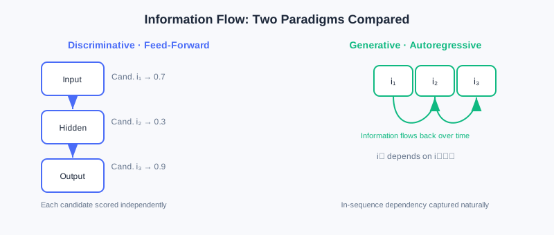
Left: a discriminative feed-forward network scoring each candidate independently; right: generative autoregression, where information flows back along time and tokens are generated one by one.
Model Architecture: Heterogeneous Specialization vs. Unified Transformer
To adapt to different stages, discriminative systems often need multiple specialized modules — two-tower or graph networks for retrieval, complex feature interaction networks for ranking, list-level constraints for re-ranking. These modules are heterogeneous and highly customized, making the system complex and costly to maintain.
Generative recommendation instead favors a unified Transformer architecture, handling all tasks through stacked self-attention and feed-forward networks. Its dense matrix computation fits GPUs/TPUs well, achieves hardware utilization (MFU) far beyond discriminative models, and enables parameter scaling (Scaling) by plain stacking.
One Level Deeper: The Difference in Modeling Philosophy
Pulling the perspective up one more level, the fundamental difference between the two paradigms lies in modeling philosophy: discriminative models pursue "making the optimal choice given a candidate set," while generative models attempt to "learn the generation process of user behavior." The former suits well-defined optimization problems; the latter is closer to the nature of human decision-making, and opens new possibilities for deeply fusing recommender systems with language models and multimodal models.
📊 Data Point: To be objective: fully end-to-end generative recommendation still faces challenges in industry today (training cost, inference latency, system stability). Research therefore proceeds along three parallel paths — ① progressive (borrowing LLM-style Scaling capability on top of cascade architectures); ② knowledge-enhanced (injecting LLM world knowledge); ③ fully generative (unifying retrieval/ranking/re-ranking into one generative model). This chapter focuses on foundations; later chapters cover each path in turn.
The interactive demo below places the two paradigms side by side, so you can step through how the same recommendation request is processed along the "discriminative scoring" path versus the "generative sequence generation" path:
⚠️ Common Mistakes in 6.1
| # | Mistake | Example | Why It's Wrong | Fix |
|---|---|---|---|---|
| 1 | Reading generative models as "scoring each candidate" | "Generative is just another way to compute CTR" | Generative models directly produce sequences; there is no per-candidate evaluation | Remember: discriminative selects, generative creates |
| 2 | Treating discriminative problems as "just bad engineering" | "A bigger model will fix the cascade" | Error accumulation / missing semantics are intrinsic to the paradigm | Understand the limitations at the paradigm level, not by stacking parameters |
| 3 | Confusing the two directions of conditional probability | Writing as and calling it generative | The former is a sequence generation distribution; the latter is per-candidate discrimination | Look carefully at which side the "condition" is on |
| 4 | Assuming generative models have no notion of a candidate set | "Generative models have no candidate space at all" | Generative models internalize the candidate space as the generation distribution; it still exists | Understand "no presupposed candidates" ≠ "no item space" |
Chapter Summary
📌 Key Takeaways
| Concept | Key Points | Why It Matters |
|---|---|---|
| Discriminative recommendation | , per-candidate scoring | The industrial mainstream — mature and stable, but with three inherent limitations |
| Three limitations | Parameter inefficiency, missing semantics, cascade dilemma | The fundamental motivation driving the paradigm shift |
| Generative recommendation | Autoregressive, end-to-end, with semantic representation built in | |
| Essential differences | Objective function / information flow / architecture | Determines whether global optimization and Scaling are possible |
| Three paths | Progressive / knowledge-enhanced / fully generative | The realistic landscape of current industrial adoption |
❓ FAQ
Q1: Is generative always better than discriminative?
A: No. Discriminative models are stable and efficient in mature scenarios; generative models have greater potential for end-to-end optimization, cold start, and semantic understanding. Both coexist in industry today — choose according to your business stage.
Q2: What exactly does autoregressive modeling solve?
A: It lets the model generate results in a single forward pass, eliminating the error accumulation and objective misalignment of multi-stage cascades; it naturally captures sequential dependencies and paves the way for end-to-end reinforcement learning.
Q3: Why is missing semantics a "paradigm problem" rather than a "data problem"?
A: The discriminative approach treats items as atomic IDs with no prior relationships, so similarity can only be "memorized" from behavioral statistics; generative models use semantic IDs so that similarity relationships are encoded in the representation structure itself, easing cold start at the root.
🔗 Connections to Later Chapters
- 6.2 (Foundations of Generative Architectures) picks up this section's "unified Transformer" claim and expands on self-attention, positional encoding, and the two architectural paradigms.
- 6.3 (LLM Foundations) systematically explains the three-stage training methodology of generative models (pretraining / instruction tuning / preference alignment).
- 6.4 (Codebook Quantization) answers the key question planted here — how generative models represent items with semantic IDs.
- 1.1 (the two paradigms) contrasts them at the intuition level; this chapter deepens the contrast to the level of modeling philosophy and architecture.
Practice Problems
Work through all problems in order — they get progressively harder. Each has a complete solution you can reveal after trying it yourself.
Problem 6.1.1 — Distinguishing Paradigms 🟢 Easy
Given the two system descriptions below, decide whether each is closer to discriminative or generative, and explain why.
- (a) The system computes a "user click probability" for every candidate ad, ranks by probability, and shows the top 5.
- (b) The system reads the user's last 20 plays and directly outputs "the 3 video IDs you might want to watch next."
💡 Solution (click to reveal)
Approach: Grasp the difference in the "questions asked" — per-candidate scoring, or directly producing a sequence.
- (a) Discriminative: it computes a click probability for each candidate separately and then ranks — exactly the "score one by one and pick the best" of .
- (b) Generative: it directly decodes a sequence of recommendation IDs from the history, without per-candidate evaluation — corresponding to .
Key points:
- Discriminative = candidates known, scored one by one; generative = directly "creates" a sequence.
- The key question: does the system enumerate and evaluate every single candidate?
Problem 6.1.2 — Listing the Three Limitations 🟢 Easy
Write down the three inherent limitations of the discriminative paradigm that are repeatedly criticized on the road toward generative models, with one sentence each on the consequence.
💡 Solution (click to reveal)
Answer:
- Parameter efficiency: embedding layers hold 90%+ of parameters yet are sparse and inefficient, keeping hardware utilization (MFU) low.
- Missing semantic modeling: items are atomic IDs with no semantic relationships, so cold start is hard to solve.
- Multi-stage cascade dilemma: stage objectives are misaligned, and information is lost at every stage (quality items wrongly filtered at retrieval are never seen again).
Key points:
- All three stem from the "per-candidate scoring + cascade" paradigm itself; engineering alone cannot erase them.
Problem 6.1.3 — Restating the Formula 🟡 Medium
The discriminative per-candidate score can be written as . Restate the core generative formula in natural language, and point out the essential difference from the discriminative case on the "conditioning" side.
💡 Solution (click to reveal)
Approach: Translate the formula piece by piece.
Answer: The formula reads: "the probability that user produces the entire interaction sequence in context equals the product over each time step of the probability of generating the -th item, conditioned on all previous interactions , the user , and the context ."
Essential difference: the discriminative "condition" is — item is given; the generative "condition" is — the item is the variable to be generated, and previous items in the sequence flow back in as conditions. The former scores candidates; the latter creates candidates from conditions.
Key points:
- The product structure = autoregression; every token depends on history.
- Whether item appears on the conditioning side is the watershed between discrimination and generation.
🏆 Challenge: Arguing a Paradigm Choice
A team must rebuild recommendations for an e-commerce scenario with "100K new items per day and a high long-tail share." In about 150 words, argue why the generative approach (semantic ID route) has more long-term value here than a purely discriminative one. Focus on "cold start, parameter efficiency, cascade information loss," and point out which discriminative components should still be kept in deployment.
💡 Hint
Long-tail / high-volume new items → atomic discriminative IDs struggle to accumulate behavior, so cold start is severe; semantic IDs let new items gain representations from content alone, and prefix generalization eases the long tail. On parameter efficiency, a unified Transformer scales more easily than heterogeneous multi-stage modules. Still, keep discriminative retrieval/re-ranking as a candidate constraint and experience safety net for the generative output, adopting a "progressive + knowledge-enhanced" hybrid path for a smooth transition.
Foundations of Generative Architectures
📝 Before You Continue: You should first read the "unified Transformer" claim in 6.1, plus the intuition about inner products and vector spaces in 2.3. This chapter does not dig into mathematical derivations; it emphasizes intuitive understanding of architectures and adaptation to recommendation scenarios.
With the core ideas of generative recommendation in place, we now build the technical foundation that supports it — the Generative Architecture. Generative recommendation models recommendation as a sequence generation task, and producing high-quality sequences requires a strong model architecture behind it.
Current generative recommendation mainly relies on two families of architectural paradigms: Transformer and Diffusion models. Their generation mechanisms are fundamentally different, yet both provide solid support for generative recommendation — Transformer generates token by token autoregressively and excels at capturing causal dependencies; Diffusion recovers data from noise through iterative denoising and offers a fresh generative perspective. More importantly, they are not mutually exclusive — they are complementary and synergistic.
After reading this chapter, you will be able to:
- Explain the Q/K/V computation and multi-head mechanism of self-attention as "query—match—aggregate"
- Explain why positional encoding (absolute/relative, time-aware) is indispensable for recommendation sequences
- Compare the strengths, weaknesses, and applicable scenarios of Encoder-Decoder vs. Decoder-Only architectures
- Explain how the causal mask enables autoregressive generation while keeping training parallel
- Outline Diffusion's forward diffusion / reverse denoising and its applications in recommendation
- Complete 5 tiered practice problems to consolidate the key mechanisms of generative architectures
6.2.0 Why Transformer and Diffusion
Since "Attention is All You Need" appeared in 2017, Transformer has become the mainstream in NLP and has expanded into vision, speech, and beyond. Its success owes not just to expressive power, but to its highly regular computation pattern — massive matrix multiplications fully exploit GPU parallelism, so training/inference efficiency far exceeds RNNs and LSTMs.
For generative recommendation, Transformer's advantages are especially pronounced:
- Long-range dependencies: self-attention naturally captures dependencies between any positions in a user behavior sequence — no matter how long the history, it can flexibly attend to signals at any moment.
- Parallel efficiency: it handles long sequences efficiently, which is crucial for modeling a user's complete behavioral history.
- Scalability: stacking more layers or widening hidden dimensions increases capacity, providing a solid basis for Scaling recommendation models.
Diffusion offers another angle: instead of building from the sequence start token by token, it starts from pure noise and gradually recovers the target through iterative denoising — like "carving a clear figure out of blurry stone." This globally parallel denoising can, in some scenarios, break through the speed bottleneck of autoregression.
6.2.1 Self-Attention: Query—Match—Aggregate
The core innovation of self-attention is letting the model focus dynamically and selectively on any position in the sequence. Its essence in one sentence: given the current Query, which parts of the sequence (Keys) are most relevant, and with what weights are their contents (Values) aggregated?
The Three-Step QKV Computation
Given an input sequence representation matrix ( sequence length, feature dimension), first apply three linear transformations to obtain Query, Key, Value:
- Query : what information the current position "wants to look up" — think of it as "the prediction need at the current moment."
- Key : what information each position of the sequence "offers" — the index used for matching against the Query.
- Value : what content each position of the sequence "actually contains" — once importance is determined, this is what gets aggregated.
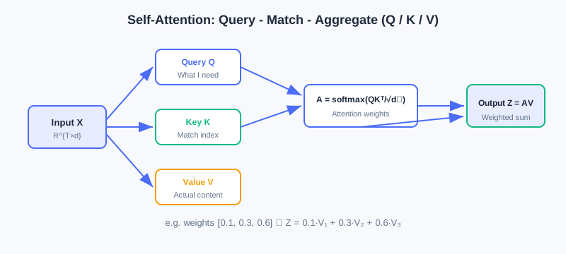
Step two computes attention weights — the inner product (similarity) of the Query with each Key, scaled and softmaxed:
The scaling factor prevents the inner products from having excessive variance when the dimension is large, which would make the softmax overly sharp (near one-hot) and drive gradients toward zero. Row of the attention matrix is "how much attention each historical position should receive when predicting the -th item."
Step three aggregates the Values by these weights:
A concrete example: with user history [item1, item2, item3], when predicting item4, the Query matches the Keys of the three items; if the attention weights are [0.1, 0.3, 0.6], the output is 0.1·V1 + 0.3·V2 + 0.6·V3 — the model extracts information from history adaptively rather than treating all history equally.
🧠 Mental Model: Multi-Head Attention as a "Panel of Experts"
A single attention head can learn only one "attention pattern." But user behavior is driven by multiple factors — sometimes price, sometimes brand, sometimes function. Multi-Head Attention computes independent Q/K/V groups in parallel; each head acts like an "expert": the 1st head might focus on "same brand" (bought an iPhone, recommend AirPods), the 2nd on "same category" (bought a phone case, recommend a screen protector), the 3rd on "recent behavior." Parallel experts let the model understand the sequence from multiple angles.
Analysis: Why not use one big single head? With heads of dimension 64, the total parameter count equals a single head of dimension 512, but multi-head lets each head learn an independent subspace and avoids mixing information — more expressive. The cost is that compute grows linearly with .
6.2.2 Positional Encoding and Time Awareness
Self-attention has a natural flaw: it is insensitive to sequence order. [item1,item2,item3] and [item3,item1,item2] produce identical outputs as long as the contents are the same. But order carries crucial temporal information in recommendation — "buy a phone first, then a case" differs in meaning from "buy a case first, then a phone." Positional Encoding exists to inject position information into every position of the sequence.
Absolute positional encoding assigns each position a fixed encoding added to the input: . The classic sinusoidal encoding
is deterministic and extrapolates; it can also be replaced by learnable positional encoding (more flexible but cannot extrapolate).
Relative positional encoding does not add encodings at absolute positions; instead, it introduces a relative position bias into the attention computation:
This generalizes better and handles variable-length sequences more naturally (BERT/GPT use absolute; T5/DeBERTa use relative).
Time Encoding Peculiar to Recommendation
User behavior sequences have not just order but also real time intervals. For example:
User A: [item1(1/1)] → [item2(1/2)] → [item3(1/3)] # dense short-term interest
User B: [item1(1/1)] → [item2(3/1)] → [item3(6/1)] # cross-month long-term interest
The orders are the same, yet the time scales differ drastically. A common approach discretizes timestamps into hour/day/week multi-granularity embeddings and sums them; more recent work like HSTU uses relative time positional encoding:
The logarithmic transform compresses the time scale so the model handles both long-term and short-term behavior well. In short-video scenarios intervals are only seconds; in e-commerce they can span weeks — choosing the right time granularity is critical for performance.
6.2.3 Two Architectural Paradigms: Encoder-Decoder vs. Decoder-Only
With self-attention and positional encoding in hand, we move to Transformer's overall architecture design. Generative recommendation mainly adopts two paradigms.
Structural Differences
Encoder-Decoder uses two towers: the Encoder processes the input (e.g., user history ) with bidirectional self-attention (each position can see all positions before and after it) to gain a global understanding; the Decoder uses two kinds of attention simultaneously — causal self-attention (predicting the -th token may depend only on the previous , ensuring autoregression) and cross-attention (Decoder hidden states as Query, Encoder outputs as Key/Value, dynamically querying input information). Representatives: the original Transformer, T5, BART; in recommendation, TIGER first introduced the T5 architecture.
Decoder-Only uses a unified single tower: input and output are treated as one continuous sequence, unified causal self-attention generates autoregressively from left to right, and generation positions can attend to all input positions and all generated positions. Representatives: the GPT series; in recommendation, HSTU, RecGPT, OneRec-V2 adopt it.
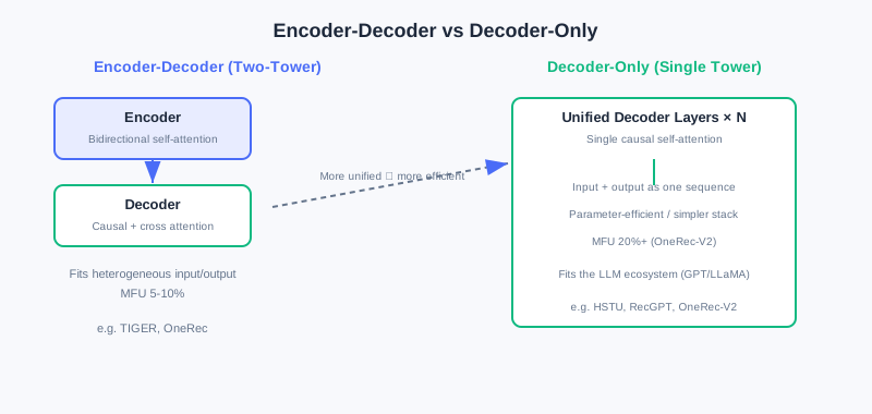
| Dimension | Encoder-Decoder | Decoder-Only |
|---|---|---|
| Attention type | Encoder bidirectional + Decoder causal + cross-attention | Unified causal self-attention |
| Parameter allocation | Spread across Encoder/Decoder/cross-attention | Concentrated in Decoder layers |
| Computation pattern | Encoder parallel encoding + Decoder autoregressive decoding | Fully autoregressive processing |
| Sequence organization | Input and output separated | Input and output concatenated |
Trade-offs
The strength of Encoder-Decoder lies in structured information processing: it decouples "understanding the user" from "generating recommendations"; the Encoder models the complete behavior sequence bidirectionally, and cross-attention provides an explicit "query—retrieve" pattern. It is especially suitable for heterogeneous input/output scenarios — e.g., multimodal inputs (behavior sequence + profile + context) and item Semantic ID sequence outputs. OneRec further splits the Encoder into short-term/long-term/positive-feedback pathways to handle different behavioral signals.
Its weaknesses are efficiency and scalability: three attention mechanisms mean more parameters and computation; cross-attention cost grows linearly with input length; scattered parameters reduce per-module capacity and limit Scaling potential.
The strength of Decoder-Only lies in simplicity and uniformity: ① high parameter efficiency — all parameters concentrate in the Decoder, so new parameters added during scaling directly strengthen core modeling; ② engineering simplicity — with only one attention type, operator fusion and memory optimization are easier, and industrial deployments reach higher MFU (OneRec-V2 achieves 20%+, versus only 5–10% for Encoder-Decoder); ③ LLM ecosystem compatibility — mainstream LLMs (GPT/LLaMA/Qwen) are all Decoder-Only, so architecture configs and training frameworks (e.g., HuggingFace Transformers) can be reused, with only the item-vocabulary Embedding reinitialized.
Its weaknesses are the unidirectional constraint (causal attention cannot see the future, sacrificing some modeling power in offline training loss) and context length pressure (no independent Encoder to compress; long behavior sequences enter whole as context). Recent work explores hybrid architectures (e.g., OneRec's Lazy Decoder sharing Encoder KV, or Decoder-Only plus bidirectional pretraining objectives) to get the best of both.
Analysis: No architecture is absolutely better. Task dimension: explicit separation of "understanding/generation" or heterogeneous modalities → Encoder-Decoder; tasks expressible as "sequence continuation" → Decoder-Only. Scale dimension: enough data to support large-scale pretraining → Decoder-Only scales better; small data and small models (<1B) → Encoder-Decoder trains more stably. Deployment dimension: under extreme latency, Decoder-Only may actually be more efficient thanks to end-to-end optimizations like KV Cache and speculative decoding.
6.2.4 Causal Masking and Diffusion Models
Causal Mask: the Key to Autoregression
Whichever architecture you choose, the causal attention mask is the key to autoregression. It applies to future positions before the softmax:
This guarantees that predicting the -th token depends only on the previous tokens, with no information leakage.
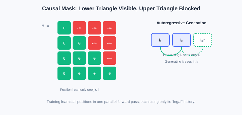
The causal mask also brings a training efficiency gain: although generation is autoregressive, training can compute the losses at all positions in parallel. Given a sequence , the model can, in one forward pass, simultaneously learn "predict from ," "predict from ," and so on — each prediction uses only "legal" history. This is a major Transformer advantage over RNNs.
Recommendation scenarios have also developed customized masks: Session-level Masking (masking across session boundaries to model multi-scenario behavior), Task-specific Masking (CTR sees the full sequence, CVR sees only the clicked subsequence), and Bidirectional Prefix Masking (static features serve as a bidirectionally visible prefix while the behavior sequence stays causal — adopted by HSTU).
Diffusion Models: A Generative View via Iterative Denoising
Unlike Transformer's token-by-token sequential generation, Diffusion models offer a new paradigm: starting from pure noise, they gradually recover the target data through iterative denoising. The core is a pair of inverse Markov processes:
- Forward diffusion: gradually add Gaussian noise to real data; after steps, obtain approximately pure noise.
- Reverse denoising: starting from random noise, a learned denoising network progressively denoises and recovers the real data.
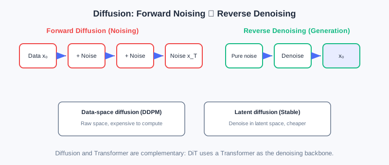
By operating space, there are two families: data-space diffusion (DDPM, directly in the raw space, computationally heavy) and latent-space diffusion (Stable Diffusion, which first compresses into a low-dimensional latent space and then diffuses — more efficient, and more commonly used in recommendation because it cuts cost while providing compact semantic representations). Conditional diffusion can further be developed, injecting conditions such as user history through concatenation/cross-attention/classifier guidance.
Diffusion applications in recommendation include: feature augmentation and representation learning (denoising in latent space to generate robust embeddings and mitigate sparsity), sequence generation (denoising an entire sequence in parallel, unconstrained by strict order), multimodal fusion, and collaborative filtering and graph-structure modeling (diffusing over latent representations of the interaction graph). The challenge is that multi-step iterative sampling brings inference latency; industrial deployment needs sampling acceleration and model distillation to balance quality and real-time performance.
💡 Key Insight: Diffusion and Transformer are complements, not rivals — many advanced Diffusion models (e.g., DiT) use Transformer directly as the denoising backbone. Generative recommendation can flexibly combine the two mechanisms per scenario: Transformer for causal dependencies and parallel Scaling, Diffusion for inherent diversity support and globally parallel generation.
⚠️ Common Mistakes in 6.2
| # | Mistake | Example | Why It's Wrong | Fix |
|---|---|---|---|---|
| 1 | Assuming self-attention perceives order natively | "Attention already contains position information" | Self-attention is order-agnostic; explicit positional encoding is required | Always add positional/time encoding |
| 2 | Ignoring the scaling factor | Softmax(QKᵀ) directly | With large , inner products have high variance; softmax gets too sharp and gradients vanish | Always divide by |
| 3 | Believing Encoder-Decoder always beats Decoder-Only | "Two towers have more complete information" | Scattered parameters limit Scaling; MFU is low | Weigh by task/scale/deployment |
| 4 | Causality leakage | No causal mask during training | Future information leaks; offline metrics are inflated | Add a lower-triangular causal mask |
| 5 | Treating Diffusion as a Transformer replacement | "Pick either one" | The two are complementary and can combine (e.g., DiT) | Combine both mechanisms per scenario |
Chapter Summary
📌 Key Takeaways
| Concept | Key Points | Why It Matters |
|---|---|---|
| Self-attention | Q/K/V query-match-aggregate, multi-head in parallel | Captures long-range dependencies, focuses adaptively |
| Positional encoding | Absolute/relative + time-aware (HSTU) | Brings order/time intervals into modeling |
| Encoder-Decoder | Bidirectional encoding + causal decoding + cross-attention | Fits heterogeneous input/output and structured modeling |
| Decoder-Only | Unified causal self-attention | Parameter-efficient, high MFU, LLM-ecosystem compatible |
| Causal mask | Lower-triangular ; training stays parallel | Guarantees both autoregressive consistency and efficiency |
| Diffusion | Forward noising / reverse denoising; latent space mainstream | Parallel generation, diversity, complementary to Transformer |
❓ FAQ
Q1: Why is time encoding more important in recommendation than in NLP?
A: "Position" in NLP is mostly syntactic order; recommendation behavior also carries real time intervals (from seconds to months), and the same order may reflect dense or long-term interest — timestamps/intervals must be explicitly encoded.
Q2: Why does Decoder-Only achieve higher MFU?
A: With only one attention mechanism, the computation pattern is highly uniform, making operator fusion and memory optimization easier — hardware utilization is significantly higher than Encoder-Decoder, where three attention mechanisms coexist.
Q3: How does the causal mask achieve "parallel training, serial generation"?
A: During training, one forward pass computes losses at all positions, but the mask lets each position see only legal history; during generation, decoding strictly proceeds step by step at .
🔗 Connections to Later Chapters
- 6.1 (paradigm foundations) proposed the "unified Transformer" claim; this chapter supplies its mechanistic details.
- 6.3 (LLM Foundations) goes deeper into Decoder-Only pretraining/fine-tuning/alignment, echoing this section's architecture choice.
- The semantic IDs of 6.4 (Codebook Quantization) are the "vocabulary" that Decoder-Only autoregressively generates.
- 7.x (Scaling) picks up this section's "stacking is scaling" and expands parameter scaling of generative models.
Practice Problems
Work through all problems in order — they get progressively harder. Each has a complete solution you can reveal after trying it yourself.
Problem 6.2.1 — Computing Attention Weights 🟢 Easy
User history [item1, item2, item3]. When predicting item4, the scaled softmax of the Query–Key inner products gives weights [0.2, 0.3, 0.5], with Values V1=[1,0], V2=[0,1], V3=[1,1]. Compute the aggregated output .
💡 Solution (click to reveal)
Approach: Weighted sum of the Values.
Key points:
- The weights sum to 1 (guaranteed by softmax).
- item3 has the largest weight, so the output is closest to V3.
Problem 6.2.2 — Role of the Scaling Factor 🟢 Easy
Let ; a Query–Key inner product is 16. Which softmax is "sharper" — without scaling, or after dividing by ? Explain the consequence.
💡 Solution (click to reveal)
Answer: Without scaling the input is 16; after scaling it is . The larger the softmax input, the sharper the distribution (approaching one-hot). Without scaling, attention would lock onto almost a single position, gradients vanish, and training struggles. After scaling, the distribution is smoother and learning is easier.
Key points:
- controls inner-product variance and prevents numerical blow-up at large dimensions.
- This is a small trick critical to stable Transformer training.
Problem 6.2.3 — Architecture Selection 🟡 Medium
A team is building a retrieval-style generative recommender with "input = user multimodal features (behavior sequence + profile + context), output = item Semantic ID sequence." Explain whether Encoder-Decoder or Decoder-Only is the better fit and why, and state one precondition under which switching to Decoder-Only would make sense.
💡 Solution (click to reveal)
Answer: Lean toward Encoder-Decoder: the input (multimodal) and output (ID sequence) are modality-heterogeneous; two towers naturally decouple "understanding the user" from "generating recommendations," and cross-attention lets the Decoder dynamically query user history. A precondition for switching to Decoder-Only: if the task can be restated as "sequence continuation" (concatenating multimodal features and history into one unified sequence and predicting subsequent items), and you pursue higher MFU, LLM-ecosystem reuse, and have enough data to support large-scale pretraining, then Decoder-Only becomes preferable.
Key points:
- Heterogeneous input/output → Encoder-Decoder wins.
- Sequence continuation + big data → Decoder-Only wins.
Problem 6.2.4 — The Causal Mask Matrix 🔴 Hard
For a sequence of length 4, write out the causal mask matrix (lower triangle 0, upper triangle ). Also explain how the model learns to predict simultaneously in "one forward pass" during training.
💡 Solution (click to reveal)
Answer:
During training, feed the full sequence ; the causal mask makes position 1 see only (learning to predict ), position 2 see (learning to predict ), position 3 see the first three (learning to predict ), and position 4 see everything but predict nothing. All position losses are computed in parallel in one forward pass, yet each uses only legal history — guaranteeing autoregressive consistency while gaining parallel efficiency.
Key points:
- Mask shape = lower triangular.
- Parallel training is the core efficiency advantage of autoregressive models over RNNs.
🏆 Challenge: Designing a Hybrid Inference Pipeline
A short-video app must generate 10 recommendations within "milliseconds" while balancing quality and diversity. In about 150 words, explain: should you adopt pure Diffusion or pure Transformer? Can they be combined? Also give two engineering techniques for compressing Diffusion inference latency.
💡 Hint
Pure Diffusion is unsuitable (multi-step iterative sampling has high latency), and neither is pure Transformer if strong diversity is required. They can be combined: use a Decoder-Only Transformer as the main generator with Diffusion for candidate augmentation/diversity completion; or DiT-style, with Transformer as the denoising backbone. Latency-compression techniques: sampling acceleration (few-step sampling/distillation), model distillation collapsing multi-step denoising into one step, plus KV Cache and speculative decoding to accelerate autoregression.
Large Language Model (LLM) Foundations
📝 Before You Continue: You should first read the Decoder-Only architecture and self-attention in 6.2. This section focuses on "how LLMs are trained," laying the groundwork for later migrating this pipeline to recommendation.
The evolution from Transformer to LLM is not just growth in parameter scale — more importantly, it is the systematization of the training paradigm. Modern LLMs (GPT-3/4, LLaMA, etc.) developed a complete "pretraining—instruction tuning—preference alignment" three-stage training pipeline, so models can generate fluent text while also understanding instructions and following human intent.
But applying LLMs to recommendation is not a matter of "plugging in" off-the-shelf language models — you must understand the modeling principles and adapt/optimize for recommendation scenarios. This section systematically introduces the basic LLM modeling pipeline, focusing on the technical links most relevant to generative recommendation.
After reading this chapter, you will be able to:
- Explain the goals and losses of each LLM stage (pretraining / instruction tuning / preference alignment)
- Distinguish the pipeline differences between RLHF (with reward model and PPO) and DPO
- Explain what Scaling Laws and emergent abilities imply for generative recommendation
- Map the three-stage paradigm to recommendation scenarios and identify challenges specific to it, such as item tokenization
- Complete 4 tiered practice problems to consolidate the LLM→recommendation knowledge chain
6.3.0 Overview of the Three-Stage LLM Paradigm
Current mainstream LLMs follow the "pretraining—instruction tuning—preference alignment" three-stage paradigm, first systematized in InstructGPT and widely adopted by GPT-4, Claude, and LLaMA. The three stages have progressive goals and together form a complete capability-building system.
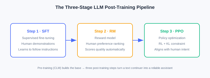
- Step 1 (SFT): collect human demonstration data for supervised fine-tuning, so the model initially learns to follow instructions.
- Step 2 (RM): collect comparison data to train a reward model that automatically evaluates output quality.
- Step 3 (PPO): with the reward model as feedback, use reinforcement learning to continually optimize the generation policy, with a KL divergence constraint to prevent drifting too far from the reference model.
🧠 Mental Model: From "Autocomplete Writer" to "Assistant"
A pretrained LLM is just a "text continuation engine" — give it an opening and it naturally keeps writing, without knowing "what you want it to do." Instruction tuning is like onboarding training (teaching it to understand task instructions); preference alignment is like values calibration (teaching it what a better answer is). Only after all three steps does it turn from a "completion tool" into a "reliable assistant."
6.3.1 Pretraining and Instruction Tuning
Pretraining: the Foundation of Language Ability
Pre-training is the first stage and the most compute-intensive. The goal is to learn general language representation and generation ability on large-scale unlabeled text, relying entirely on self-supervised learning (the data itself provides the signal; no manual annotation needed).
Training objective: causal language modeling (CLM), also known as Next Token Prediction:
where . By maximizing this likelihood, the model masters the statistical regularities of language, grammar, semantics, and even commonsense reasoning.
When model scale and data scale reach a certain level, Scaling Laws emerge: performance keeps improving with parameter count, data volume, and compute, and Emergent Abilities such as zero-shot/few-shot learning may even appear.
Analysis: Most modern LLMs use Decoder-Only architectures (GPT/LLaMA) — clean, efficient, and well-suited to large-scale training. Parameters range from billions to trillions (GPT-3 175B, PaLM 540B, LLaMA-2 7B–70B, GPT-4 estimated over 1T). Pretraining needs thousands to tens of thousands of GPUs/TPUs for weeks to months at extreme cost — so most teams fine-tune directly on open pretrained models (LLaMA, Mistral).
Instruction Tuning: Following Instructions
A pretrained model only "completes text" — it does not "understand and execute instructions." Instruction Tuning, also called Supervised Fine-Tuning (SFT), addresses "making the model understand task instructions and generate accordingly."
The core is constructing "instruction—input—output" triples, for example:
Instruction: Summarize the main content of the following passage.
Input: [a passage about the history of artificial intelligence]
Output: [Artificial intelligence started in the 1950s ... and has gone through several stages of development ...]
Training objective: conditional language modeling loss, computed only on the output portion:
where is the conditioning information (instruction + input) and is the target output. Key point: the loss is computed only on output tokens — instruction and input do not participate in gradient updates. Either full fine-tuning or parameter-efficient methods (e.g., LoRA) can be used. SFT models significantly outperform pure pretrained models on zero-shot/few-shot tasks — they have learned the meta-ability of "understanding instructions."
6.3.2 Preference Alignment and From LLM to Recommendation
Preference Alignment: RLHF and DPO
Even after instruction tuning, LLM outputs can still be insufficiently helpful, hallucinated, or unsafe. The root cause is that SFT only learns "how humans would answer," without optimizing "which answer is better." Preference Alignment makes outputs better match human values and preferences.
RLHF (Reinforcement Learning from Human Feedback) proceeds in three steps:
- Collect preference data: for the same prompt, the model generates multiple outputs; human annotators rank them, yielding preference pairs ( chosen, rejected).
- Train the reward model (RM):
- Policy optimization (PPO): maximize the reward while constraining deviation from the reference model with KL divergence:
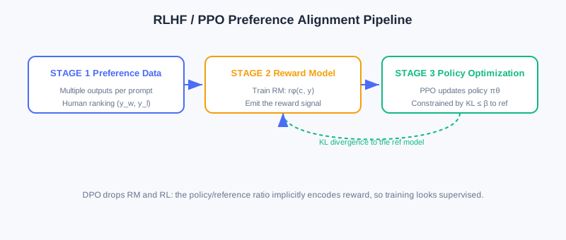
DPO (Direct Preference Optimization) is more concise: its core idea is that "the reward model can be represented implicitly by the policy model itself" — no explicit RM training and no reinforcement learning:
DPO training resembles supervised learning — simple and stable, often matching or exceeding RLHF, and widely adopted recently.
Mapping the Three-Stage Paradigm to Recommendation
The LLM's three stages provide a complete capability framework for recommendation, but each stage needs repositioning:
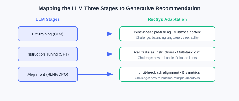
| LLM Stage | Recommendation Adaptation Direction | Core Challenge |
|---|---|---|
| Pretraining | User behavior sequence pretraining, multimodal content pretraining | How to represent items? How to balance language ability and recommendation ability? |
| Instruction tuning | Instructionalizing recommendation tasks, multi-task joint training | How to design recommendation instructions? How to handle ID-based items? |
| Preference alignment | Implicit feedback alignment, business metric optimization | How to construct preference data? How to balance multiple objectives? |
- Pretraining: the core is "letting the model master both language understanding and recommendation modeling." Overemphasizing language neglects collaborative signals; over-focusing on behavior weakens semantics — a balance is needed: for content items (news/video), language ability matters more; for collaboration-rich domains (e-commerce/music), behavior modeling matters more.
- Instruction tuning: the difficulty is that items exist as IDs, which are completely alien symbols to a language model. These IDs must be "translated" into semantic representations the model understands — this is exactly the core of item tokenization, the key bridge connecting traditional recommendation data and generative models (see Section 6.4).
- Preference alignment: recommendation feedback is mostly implicit (clicks, watch time, skips), and objectives are often multi-dimensional (CTR, retention, ecosystem health). Constructing effective preference signals from implicit feedback and balancing multiple metrics is subtler than in LLMs.
Challenges Specific to Recommendation Scenarios
Beyond adapting the three stages, generative recommendation must face four families of challenges rarely seen in the LLM domain:
- Item tokenization: natural language tokens carry semantics by construction; recommendation item IDs are abstract numbers, meaningless to the model. How to inject semantics and characterize similarity between IDs? — the core topic of Section 6.4.
- Collaborative signal fusion: "users who bought A also buy B" cannot be obtained from textual descriptions; careful design is needed to inject collaborative signals into generative architectures.
- Cold start: new items/new users lack interactions; generative models can leverage LLM semantic understanding to build capability quickly from content features, but the model must be trained to adaptively switch — "collaboration when interactions exist, content when they don't."
- Real-time constraints: online services often must respond within tens of milliseconds; autoregressive token-by-token generation can take hundreds of milliseconds. Inference optimizations (quantization, KV Cache, speculative decoding) and system-level innovations (hybrid architectures, offline-online combination, caching) are needed.
💡 Key Insight: Generative recommendation is not "wrapping a language model around recommendation" — it is reconceptualizing recommendation as a sequence generation problem and deeply adapting to recommendation's unique characteristics. It borrows the successful LLM paradigm while creatively solving recommendation-specific challenges — this chain of knowledge is the foundation for later chapters (Scaling architectures, end-to-end generation, thinking recommenders, diffusion models).
⚠️ Common Mistakes in 6.3
| # | Mistake | Example | Why It's Wrong | Fix |
|---|---|---|---|---|
| 1 | Computing the SFT loss on all tokens | Instructions also get gradients | SFT computes the loss only on outputs; input/instruction are conditions | Loss applies only to |
| 2 | Assuming RLHF needs no reference model | Just maximize the reward directly | The model learns to "game" the reward model; quality degrades | Add a KL constraint toward |
| 3 | Confusing RLHF and DPO complexity | "Both need a reward model" | DPO represents the reward implicitly; no explicit RM/RL needed | DPO training resembles supervised learning |
| 4 | Applying the LLM vocabulary to items directly | "Encode products with an off-the-shelf tokenizer" | Item IDs are alien symbols to an LLM | Item tokenization is required (see Section 6.4) |
| 5 | Ignoring multi-objective preference alignment in recommendation | "CTR as the reward is enough" | Implicit feedback + multiple objectives need careful construction | Handle multi-objectives and implicit signals explicitly |
Chapter Summary
📌 Key Takeaways
| Concept | Key Points | Why It Matters |
|---|---|---|
| Pretraining CLM | The foundation of general generation ability; Scaling Law emergence | |
| Instruction tuning SFT | Conditional language modeling; loss only on outputs | From "completion" to "following instructions" |
| RLHF | RM + PPO + KL constraint | Value alignment, but a complex pipeline |
| DPO | Implicit reward; resembles supervised training | Simple and stable; the recent mainstream |
| Recommendation mapping | Three stages → behavior pretraining / task instructionalization / implicit alignment | Each stage needs repositioning |
| Four challenges | Tokenization / collaboration / cold start / real-time | Determines whether research can reach production |
❓ FAQ
Q1: Why is DPO simpler than RLHF yet often more effective?
A: DPO merges "training a reward model + reinforcement learning" into one step — the reward is represented implicitly by the ratio of policy to reference model, training looks like ordinary supervised learning, and it avoids RL's instability and the extra RM.
Q2: Why is preference alignment harder in recommendation?
A: LLMs have explicit human preference rankings; recommendation feedback is mostly implicit behavior (clicks/skips), objectives are multi-dimensional and often conflict, so constructing the "what is better" signal is subtler.
Q3: What do Scaling Laws mean for recommendation?
A: Like LLMs, generative recommendation models keep improving with parameters/data/compute — which supports the "stacking is scaling" claim of [6.2] and the later Scaling chapters.
🔗 Connections to Later Chapters
- The Decoder-Only architecture of 6.2 (architectural foundations) is exactly the main architecture for LLM pretraining.
- 6.4 (Codebook Quantization) solves the "item tokenization" bridge problem raised repeatedly in this section.
- 8.x (End-to-end Generation) implements the three-stage paradigm in recommendation training pipelines.
- 9.x (Thinking Recommenders) deepens the combination of preference alignment and reasoning-style generation.
Practice Problems
Work through all problems in order — they get progressively harder. Each has a complete solution you can reveal after trying it yourself.
Problem 6.3.1 — Scope of the SFT Loss 🟢 Easy
An instruction tuning sample: instruction "Translate into English", input "Bonjour le monde", output "Hello world". If the output is tokenized into 2 tokens, which tokens should the training loss cover? Do the instruction and input tokens participate in gradient updates?
💡 Solution (click to reveal)
Answer: The loss covers only the output tokens Hello and world (2 tokens), computing at each position. The instruction "Translate into English" and the input "Bonjour le monde" serve as conditions and do not participate in gradient updates — the model learns only "given instruction + input, how to generate the correct output."
Key points:
- Conditional language modeling: conditions are fixed; the loss applies only to outputs.
- This is the key difference between SFT and pretraining CLM.
Problem 6.3.2 — Reward Model Loss 🟢 Easy
For a preference pair , the reward model gives . Compute the RM loss term and explain what it encourages.
💡 Solution (click to reveal)
Approach: Substitute values.
; ; loss term .
Answer: This small loss (near 0) indicates the reward model already scores higher. The RM loss overall encourages "giving higher reward scores to better outputs," enabling the RM to automatically evaluate the quality of any output.
Key points:
- compresses score differences into a probability.
- The RM learns "relative better/worse," not absolute scores.
Problem 6.3.3 — RLHF vs. DPO 🟡 Medium
Briefly describe the differences between RLHF and DPO on three aspects: "whether an explicit reward model is needed," "whether reinforcement learning is used," and "training stability."
💡 Solution (click to reveal)
Answer:
| Dimension | RLHF | DPO |
|---|---|---|
| Explicit reward model | Needed (train an RM separately) | Not needed (reward represented implicitly by the policy/reference ratio) |
| RL used | Uses PPO reinforcement learning | No — training resembles supervised learning |
| Training stability | Lower (RL is unstable, easy to game the RM) | Higher (no RL, no separate RM) |
Key points:
- DPO replaces RM + RL with the reference model .
- DPO has recently been favored for being simple, stable, and comparably effective.
🏆 Challenge: Designing Preference Alignment for Recommendation
A music app wants to optimize recommendations with preference alignment but has only implicit signals (play completion rate, favorites, skips). In about 150 words, explain: how would you construct preference pairs from implicit behavior? Which business objectives must be balanced (list at least 2)? And state the essential difference from LLMs' explicit rankings.
💡 Hint
Construction: generate multiple candidate sequences for the same user and context, and define quality via implicit signals — e.g., with high completion rate and a favorite; with many skips / low completion. Objectives to balance: user retention, content ecosystem health (diversity/long tail). Essential difference: LLMs have explicit human rankings, while recommendation infers preferences from behavioral proxies — noisier, with often-conflicting multi-objectives requiring weighting, not a plain "good/bad binary classification."
Tokenizer Technology in Recommendation: Codebook Quantization and Semantic IDs
📝 Before You Continue: Please first read the "item tokenization" problem raised repeatedly in 6.3, and the Decoder-Only autoregressive generation in 6.2 — semantic IDs are exactly the "vocabulary" fed to it.
In [6.3] we pointed out that Item Tokenization is the key bridge connecting traditional recommendation data and generative models. This chapter faces this core problem head-on: how do we transform items in a recommender system into token sequences that generative models can understand and generate?
After reading this chapter, you will be able to:
- Compare the strengths and weaknesses of the three paradigms: sparse ID / text ID / semantic ID
- Explain the three values of semantic IDs: "controlled vocabulary, hierarchical structure, from memorization to reasoning"
- Derive VQ-VAE's quantization and three losses, and understand the Straight-Through Estimator (STE)
- Explain how RQ-VAE's residual quantization produces hierarchical semantic IDs
- Know industrial-grade decoupled and hybrid schemes such as RQ-Kmeans / RQ-OPQ
- Complete 5 tiered practice problems and experience quantization hands-on with the interactive demo
6.4.0 The Evolution of Three Tokenizer Paradigms
Understanding the three mainstream item representation paradigms is both a technology choice and a shift in modeling philosophy.
The Sparse ID Paradigm (Sparse ID-Based)
The traditional approach: assign each item a unique atomic ID (e.g., item_10086). In discriminative models, the ID is mapped to a continuous vector through an embedding layer, and a deep network then learns interactions. Representatives: HSTU (organizing behavior into structured sequences like [item, action, timestamp, ...]), GenRec (using sparse IDs directly in a generative architecture).
Advantages: collision-free guarantee, freedom in feature interaction, mature engineering.
But migrating this to generative models faces three fundamental dilemmas:
- Vocabulary explosion: generative models do next-token prediction over a vocabulary, with Softmax complexity . GPT-3's vocabulary of about 50K and LLaMA's 32K are tolerable; but with billions of videos on short-video platforms and hundreds of millions of products on e-commerce sites, vocabularies reach the billion scale — far beyond what Softmax can bear.
- The dual dilemma of storage and generalization: maintaining 256-dim embeddings for a billion IDs takes roughly 1TB of parameters; more fatally, atomic IDs are orthogonal — a new item is an alien symbol to the model and must accumulate data from zero before it is "recognized."
- Implicit dependence on collaborative signals: ID similarity can only be learned from massive behavioral statistics like "watched A, also watched B"; with sparse data it degrades sharply.
The Text ID Paradigm (Text-Based)
Since LLMs excel at natural language, why not represent items as text? Serialize attributes/descriptions into natural language and encode/generate with the LLM's pretrained vocabulary (30–50K). Representatives: M6-Rec (filling attributes into templates as text), LLMTreeRec (tree-structured hierarchical text), TallRec/P5 (key-value pairs reusing T5).
Advantages: rich semantics, zero-shot generalization, strong interpretability.
Two fatal flaws:
- Low representation efficiency: one product takes tens to hundreds of tokens (an iPhone example runs about 30 tokens); self-attention's cost grows quadratically with length, and information density is sparse.
- Grounding difficulty: how does generated text map precisely back to the candidate set? There are ambiguities ("Apple phone" matches hundreds of models), incompleteness, and out-of-candidate-set issues. BIGRec patches this with two stages + L2 re-ranking, but that betrays the original end-to-end intent.
The Semantic ID Paradigm (Semantic ID-Based)
The Semantic ID (SID) is a revolutionary leap beyond the previous two: items are represented as fixed-length discrete token sequences, where each token comes from a controllably sized semantic codebook (thousands to tens of thousands). Taking TIGER as an example, a video of "NBA superstar dunk highlights" is encoded as:
SID = [10, 5, 42] # sports → basketball → dunk highlights
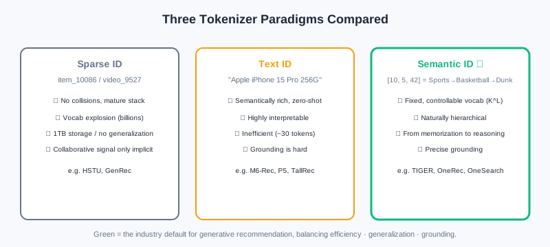
Three core advantages:
- Controlled fixed vocabulary: no matter how large the item catalog, the base semantic units are limited. With vocabulary and sequence length , the theoretical capacity is items — far beyond any real catalog. OneRec uses a vocabulary of about 8000 and OneSearch 4000–6000, keeping end-to-end autoregressive training costs manageable.
- Naturally hierarchical structure: an SID is a hierarchical sequence — prefixes are coarse-grained ("sports"), suffixes fine-grained ("basketball dunks"). It naturally supports prefix matching — first settle the category, then refine, consistent with human cognition; similar items share prefixes, providing a structured inductive bias.
- The leap from memorization to reasoning: atomic IDs can only "memorize" associations; semantic IDs encode similarity relationships in the token structure — all basketball videos share the
[10,5,...]prefix. Once the model learns that a user likes "basketball" as a semantic, it generalizes to all new items containing that token, even if they never appeared in training data.
💡 Key Insight: Semantic IDs elegantly balance the conflicting demands of representation capacity, computational efficiency, and precise grounding — the mainstream choice for current industrial generative recommendation — processable efficiently by LLMs while retaining the collaborative information recommendation depends on.
6.4.1 The Design Philosophy from Atomic IDs to Semantic IDs
Traditional atomic IDs (ID:10086) work well in discriminative architectures — the embedding layer maps the ID to a continuous vector, and massive behavior draws the vectors of two Jackie Chan action films close together. But once reframed as a generative problem, it is fundamentally incompatible with generative architectures: generative models require probabilistic modeling over a discrete token space, and an atomic ID's ultra-large vocabulary makes this infeasible both mathematically and engineering-wise.
The core idea of semantic IDs is to shift items from "identity markers" to "semantic descriptions" — instead of random numeric labels, a sequence of meaning-bearing tokens represents content attributes. Analogy: you wouldn't say "recommend ID:89757"; you'd say "recommend a sci-fi thriller about AI awakening with stunning visuals" — this description uniquely identifies the film through hierarchical concept composition (sci-fi → thriller → AI → visuals) and naturally encodes similarity (all sci-fi films share the "sci-fi" prefix).
In engineering practice, semantic IDs integrate two families of signals:
- Content signals: multimodal features (visuals/title/images) are turned into semantic vectors by pretrained encoders (CLIP, BERT).
- Collaborative signals: the crowd behavior patterns contained in the user-item interaction matrix.
The two are jointly encoded into a continuous semantic vector, then converted into a token sequence via discretization encoding (vector quantization), e.g., "NBA dunk highlights" → [sports, basketball, dunk, highlights] → numbers [10, 5, 42, 89].
Fundamental Improvements on Three Levels
- Controlled fixed vocabulary: from the combinatorial nature of sequences — a limited set of base units composes to represent massive item catalogs.
- Hierarchical structure: vertical (coarse → fine progression) + horizontal (similar items at the same level cluster together). Once the model learns a user likes token 5 (basketball), it naturally transfers to all
[10,5,...]items — prefix-based generalization. - From memorization to reasoning: first-order reasoning (item B with the same prefix resembles A), second-order reasoning (cross-category transfer "basketball → soccer"), compositional reasoning ("tutorial + basketball" → basketball tutorial videos). It stays strong under cold start/long tail — the fundamental reason semantic IDs became mainstream.
6.4.2 VQ-VAE: The Foundation of Discretization
VQ-VAE (Vector Quantised-VAE) is the foundational technique for semantic ID discretization, solving the key problem of "converting continuous high-dimensional semantics into discrete symbol sequences while preserving representational power." It introduces a learnable Codebook, establishing an effective mapping from continuous semantic space to discrete symbol space — dramatically reducing dimensionality (billions of atomic IDs → a codebook of tens of thousands) while giving IDs semantic relationships.
Three-Stage Architecture
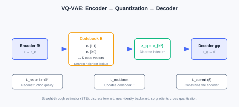
① Encoder mapping: the encoder maps input to a continuous latent vector ( achieves dimensionality reduction).
② Vector quantization: maintain a learnable codebook ( from thousands to tens of thousands); quantization is nearest-neighbor search:
This discretizes the continuous into codebook index . Numerical walkthrough: if , codebook and , then the distance to is and to is — choose , i.e., : the continuous space "collapses" onto the nearest discrete point.
③ Decoder reconstruction: . Overall: .
Loss Function (Three Cooperative Parts)
- Reconstruction loss : measures reconstruction quality ( for images, cosine for text).
- Codebook loss : uses (stop-gradient) to pull codebook vectors toward encoder outputs; gradients update only the codebook , not the encoder.
- Commitment loss ( recommended 0.25): constrains encoder outputs from straying far from the quantized codeword, preventing training instability.
Gradient Propagation: the Straight-Through Estimator (STE)
The quantization is non-differentiable almost everywhere, so standard backpropagation fails. VQ-VAE uses the STE: the forward pass strictly performs discretization; the backward pass treats quantization as an identity mapping, , passing decoder gradients straight back to the encoder. Gradient flow: the encoder receives reconstruction (via STE) + commitment gradients; the decoder receives only reconstruction gradients; the codebook receives only codebook-loss gradients.
Analysis: Note that although VQ-VAE has "VAE" in its name, it is essentially different from a variational autoencoder — it directly optimizes reconstruction loss and uses a discrete codebook for representation learning, closer to an ordinary autoencoder, and introduces no KL-constrained ELBO.
6.4.3 RQ-VAE: Hierarchical Residual Quantization
VQ-VAE maps each item to a single discrete token, facing a "representation precision vs. codebook size" trade-off: increasing improves precision but destabilizes training; decreasing leaves a single token unable to capture complex multi-dimensional semantics.
RQ-VAE (Residual Quantised-VAE) fundamentally breaks this limit with residual quantization: it expands single quantization into an -layer cascade, each layer capturing what the previous layer missed, producing a token sequence of length . Codebook size stays controlled at , while theoretical representation capacity rises to .
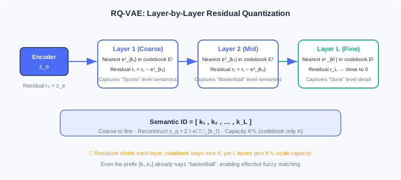
The Residual Quantization Iteration Mechanism
Given the encoder output , at layer ():
where ; the final quantized representation is , and the semantic ID is the token sequence .
Numerical walkthrough (residual approximation): target (1-dimensional), two codebook layers. Layer-1 codebook : nearest is , residual ; Layer-2 codebook : nearest is , residual . Reconstruction ; the error drops from 0.5 to 0.1.
Hierarchical semantics emerge: layer-by-layer approximation naturally forms a hierarchy — early layers capture coarse granularity ("sports"), later layers fine granularity ("basketball tutorials"). Take "NBA superstar dunk highlights" as an example:
- Layer 1 (coarse): closest to is "sports" , ID=
[10]; the residual still contains "which sport?" - Layer 2 (medium): closest in the residual is "basketball" , ID=
[10,5]; the residual focuses on "game or tutorial? dunk or jump shot?" - Layer 3 (fine): "dunk action" captures the detail; the final
SID=[10,5,42].
This "continuous focusing" mechanism means that seeing only the prefix [10,5] already tells the model it is a basketball video, achieving effective fuzzy matching.
Loss and Gradients
The RQ-VAE loss extends VQ-VAE's to a multi-layer accumulation:
Each layer independently optimizes its own codebook , with the commitment loss cascading to prevent residual drift. Gradients still rely on the STE, applied independently at each layer's quantization point.
The interactive demo below lets you intuitively experience how RQ-VAE quantizes an item vector layer by layer and produces a hierarchical semantic ID:
Click "Next step" to observe: the encoder output → Layer-1 quantization capturing coarse semantics → the residual passed to the next layer → progressive refinement until the complete SID sequence is produced. Notice how each layer's residual gets smaller and smaller.
6.4.4 Industrial-Grade Solutions: Decoupling and Hybrid
End-to-end RQ-VAE training has maintenance difficulties in large-scale industrial deployment: every model update requires recomputing SIDs for all items. Hence two-stage solutions based on decoupling emerged.
RQ-Kmeans: Decoupled Clustering
RQ-Kmeans proposes: a codebook is essentially a clustering partition of representation space — why not build it directly with K-means? It decouples discretization into two steps: ① any representation model (BERT/CLIP) produces continuous item vectors; ② K-means clustering directly on those vectors builds the codebook. The representation model and the codebook can iterate independently; quantizing a new item needs only vector search, no retraining.
The residual quantization framework is retained, but gradient learning is replaced by K-means: at layer , cluster the residual set to get codebook ; assign each item its nearest centroid index , and pass the residual to the next layer. Finally , with quantized representation .
The core difference from RQ-VAE is that representation learning is decoupled from codebook construction — new items can be quickly assigned SIDs via Faiss vector search, and K-means' uniform clustering also naturally mitigates "codebook collapse."
RQ-OPQ: Hybrid Encoding
RQ-VAE/RQ-Kmeans share a key problem: the last layer's residual is discarded outright, yet it contains unique attributes (specific brand and model, price range) — precisely what distinguishes similar items in e-commerce search.
RQ-OPQ proposes a hybrid scheme: RQ handles hierarchical semantics, while OPQ (Optimized Product Quantization) handles horizontal unique attributes. OPQ first learns a rotation matrix that projects the residual into a subspace that is easier to quantize, then splits it into sub-vectors for independent scalar quantization; the subspace indices are concatenated into the OPQ tokens (an implicit codebook of ). With OneSearch's configuration , this yields a representation space of .
Complete encoding: RQ-Kmeans gives hierarchical tokens and the final residual ; OPQ encodes into supplementary tokens . Finally
OneSearch actually uses (4096,1024,512 | 256,256): 3 layers of RQ-Kmeans + 2 layers of OPQ, 5 tokens per item. Take the iPhone 15 (pink, 256GB): the RQ part [102,8,1] (electronics → mobile phones → Apple) establishes the hierarchical identity; OPQ encodes "pink" and "256GB" from the residual as [56,99]. The final [102,8,1,56,99] contains both the phone's hierarchical facts and the specific SKU's unique attributes — perfectly resolving long-tail product distinction and retrieval.
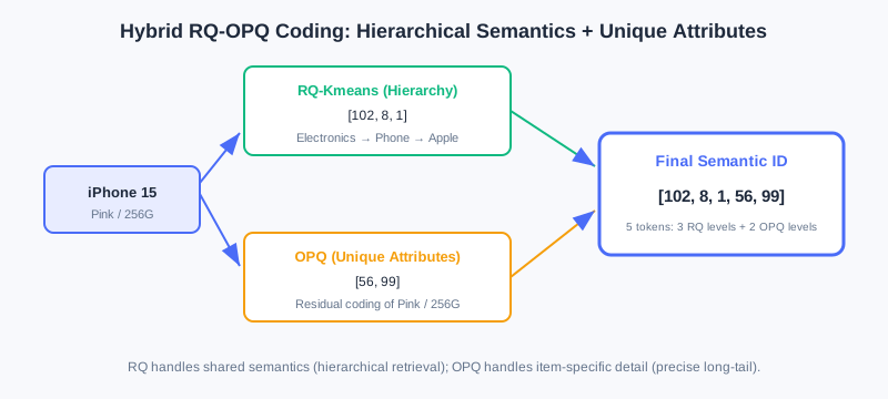
Core Challenges and Responses
| Challenge | Root Cause | Response Strategy |
|---|---|---|
| SID collisions | Quantization clustering's "uneven codebook utilization" maps multiple items to the same SID | Optimize at training time (uniform allocation, capacity limits) + remedy at inference (hybrid encoding disambiguation) |
| Objective misalignment | Representation extraction / SID quantization / generation training are optimized independently in three stages, lacking end-to-end alignment | Joint optimization (end-to-end gradients) + self-supervised alignment (cycle consistency, iterative adaptation) |
| Multimodal fusion | Content/collaborative/context modalities have inconsistent distributions; naive concatenation fails | Fusion at the representation layer (gating/contrastive learning) + fusion at the quantization layer (modality-specific codebooks, MoE) |
⚠️ Common Mistakes in 6.4
| # | Mistake | Example | Why It's Wrong | Fix |
|---|---|---|---|---|
| 1 | Using item IDs directly as the generative vocabulary | "Softmax over a billion products directly" | Vocabulary explosion; Softmax is unaffordable | Use semantic IDs to compress into a controlled vocabulary |
| 2 | Believing text IDs are a panacea | "Just describe items in natural language" | Low representation efficiency + grounding difficulty | Semantic IDs balance efficiency and precise mapping |
| 3 | Confusing VQ-VAE with VAE | "VQ-VAE uses a KL-constrained ELBO" | VQ-VAE has no variational inference; it is direct reconstruction | Remember it is an autoencoder with a codebook |
| 4 | Ignoring the straight-through estimator | "Quantization can be backpropagated directly" | is non-differentiable almost everywhere | Use the STE to pass gradients as if identity |
| 5 | Discarding the RQ's last-layer residual | "The residual is useless, drop it" | The residual holds unique attributes, key to long-tail distinction | RQ-OPQ encodes the residual with OPQ |
Chapter Summary
📌 Key Takeaways
| Concept | Key Points | Why It Matters |
|---|---|---|
| Three paradigms | Sparse ID / text ID / semantic ID | Semantic IDs balance efficiency · generalization · grounding |
| Semantic ID value | Controlled vocabulary / hierarchy / from memorization to reasoning | The mainstream industrial choice |
| VQ-VAE | Encoder-quantizer-decoder + three losses + STE | The foundation of discretization |
| RQ-VAE | Residual quantization → hierarchical SIDs; capacity | Breaks the single-token representation bottleneck |
| RQ-Kmeans | K-means replaces gradient-learned codebooks; decoupled | New items need no retraining |
| RQ-OPQ | RQ hierarchy + OPQ unique attributes hybrid | Precise distinction of long-tail products |
❓ FAQ
Q1: Why do semantic IDs ease cold start?
A: Similar items share semantic prefixes (like
[10,5,...]); once the model learns the "basketball" preference, it generalizes to all new items containing that token — no need to memorize from behavioral data.
Q2: What does RQ-VAE add over VQ-VAE?
A: Residual quantization upgrades a single token to an -layer token sequence; codebook size is unchanged but capacity rises to , and hierarchical semantics emerge naturally.
Q3: Why does industry prefer RQ-Kmeans over end-to-end RQ-VAE?
A: End-to-end requires recomputing the whole catalog's SIDs on every update; RQ-Kmeans decouples representation from the codebook — new items get SIDs via vector search, and K-means' uniform clustering mitigates codebook collapse.
🔗 Connections to Later Chapters
- The Decoder-Only autoregression of 6.2 (architectural foundations) is exactly the "generator" that consumes semantic ID sequences.
- 6.3 (LLM Foundations) listed "item tokenization" as the core migration challenge; this chapter delivers the solution.
- 8.x (End-to-end Generation) uses SIDs as the input/output interface of models like TIGER/OneRec.
- The latent-space diffusion of 10.x (Diffusion Recommendation) shares the space-compression idea with this section's codebook quantization.
Practice Problems
Work through all problems in order — they get progressively harder. Each has a complete solution you can reveal after trying it yourself.
Problem 6.4.1 — Vocabulary Capacity Computation 🟢 Easy
Let the semantic ID codebook size be and the sequence length . How many distinct items can be represented in theory? Contrast this with the embedding scale the sparse ID paradigm would need to maintain for the same number of items (256 dims per item, float32).
💡 Solution (click to reveal)
Approach: Combinatorial property.
items.
Sparse IDs would need bytes bytes exabytes (EB) — utterly infeasible; semantic IDs need only codebook vectors (each 256-dim float32 codeword is about 1KB, so all 32000 codewords total roughly 32MB).
Key points:
- Semantic IDs express massive catalogs with "combinations of short sequences" under a controlled vocabulary.
- This is exactly the key to solving vocabulary explosion.
Problem 6.4.2 — VQ-VAE Quantization 🟢 Easy
The encoder output is , codebook . Find the quantization index and , and explain how the STE approximates in the backward pass.
💡 Solution (click to reveal)
Approach: Nearest neighbor.
Distance to : ; distance to : . Choose , so , .
In the backward pass, the STE treats quantization as identity: — gradients pass straight through the discrete jump back to the encoder.
Key points:
- Forward strictly discrete, backward approximated as identity.
- The STE is standard equipment for training VQ-family models.
Problem 6.4.3 — RQ-VAE Residuals 🟡 Medium
Target ; Layer-1 codebook selects ; Layer-2 codebook selects . Write out each layer's residual and the final reconstruction , and explain how hierarchical semantics emerge.
💡 Solution (click to reveal)
Answer:
- Layer 1: (representing the "integer scale"), .
- Layer 2: (representing the "fractional part"), .
- Reconstruction , error (down from ).
Hierarchical semantics: layer 1 captures the coarse granularity (overall scale/major category), layer 2 captures fine granularity (residual details); layer-by-layer refinement is "continuous focusing," and the sequence [5, 0.4] itself carries a coarse-to-fine structure.
Key points:
- The residual = information the previous layer failed to capture, passed to the next layer.
- Stacking layers multiplies capacity to , with natural hierarchy.
Problem 6.4.4 — Why RQ-OPQ Is Necessary 🔴 Hard
Explain why the RQ's last-layer residual should not be discarded, and write out the structure of the final RQ-OPQ ID. Use the iPhone 15 (pink, 256GB) to explain the division of labor between RQ and OPQ.
💡 Solution (click to reveal)
Answer: The RQ residual contains an item's unique attributes (brand/model, price, color) — precisely what distinguishes similar items in e-commerce search; discarding it makes precise distinction of long-tail products impossible.
Final RQ-OPQ ID:
iPhone 15 (pink, 256GB): the RQ part [102,8,1] = electronics → mobile phones → Apple, establishing the hierarchical identity (grouped with Huawei/Xiaomi under "phones"); OPQ encodes "pink" and "256GB" from the residual as [56,99], dedicated to precisely matching the user's specific attribute constraints. The final [102,8,1,56,99] holds both hierarchical facts and SKU uniqueness.
Key points:
- RQ handles shared semantics; OPQ handles individual characteristics.
- Hybrid encoding balances retrieval (hierarchy) and precision (uniqueness).
🏆 Challenge: Designing an SID Scheme
An e-commerce platform has 500M products with 500K new additions per day. In about 150 words, explain: should you choose end-to-end RQ-VAE or decoupled RQ-Kmeans? Give a vocabulary and layer-count configuration approach, and point out how to handle "SID collisions" and "new items going live without retraining the whole catalog."
💡 Hint
Choose decoupled RQ-Kmeans: with 500K daily additions, end-to-end RQ-VAE would require recomputing all 500M SIDs — cost explodes; after decoupling, new items get SIDs via vector search (Faiss) with no retraining. Configure e.g. 3 RQ layers + 2 OPQ layers (referencing OneSearch), codebooks around 4096–8000. Mitigate SID collisions with uniform allocation/capacity-limiting algorithms; disambiguate the long tail via OPQ unique attributes; new items only need vector search, no entry into training.
Traditional deep learning recommendation models (DLRMs) have long been the "exception" to deep learning Scaling Laws: throw in more parameters and more data, and metrics plateau almost immediately. This part follows the thread from Meta's HSTU — the first validation of the Scaling Law in recommender systems — and then unpacks the follow-up work from Xiaohongshu, Meituan, Alibaba, and ByteDance, so you can see how industry turned "generative ranking" from paper numbers into a reality serving billions of users.
What This Part Covers
| Section | Topic | The Big Idea |
|---|---|---|
| 7.1 | HSTU: The First Exploration of the Scaling Law | Treat user behavior history as a "language"; a unified sequence + autoregressive training + an efficient architecture prove for the first time that recommendation can scale |
| 7.2 | The Overall Generative Ranking Paradigm (GenRank) | The autoregressive mechanism is what is essential; Action-Oriented sequence organization halves sequence length and speeds up training by ~79% |
| 7.3 | MTGR: Hybrid Paradigm Modeling | Use a "generative architecture + discriminative objective" to retain cross features, solving the missing-feature problem of pure generative approaches |
| 7.4 | RankMixer: Hardware Efficiency Optimization | Derive the architecture from GPU hardware characteristics; Token Mixing / Per-Token FFN / Sparse MoE push MFU from 4% to 45% |
| 7.5 | OneTrans: A Unified Transformer | A single Transformer backbone does both sequence modeling and feature interaction, and reuses LLM system optimizations such as KV Caching |
What You'll Be Able to Do After This Part
- 🟢 Explain why traditional DLRMs struggle to scale, and how HSTU broke through the bottleneck with user-level sequence modeling
- 🟢 Distinguish the respective contributions of the "autoregressive mechanism" versus "training paradigm details" within the generative paradigm (see Section 7.2)
- 🟡 Explain how MTGR's hybrid paradigm stays compatible with traditional cross features while retaining efficiency (see Section 7.3)
- 🟡 Analyze how RankMixer's hardware-aware design raised MFU from 4% to 45% (see Section 7.4)
- 🔴 Recount how OneTrans achieves end-to-end scalability with a unified Transformer + Pyramid Stack + Cross-Request KV Caching (see Section 7.5)
- 🔴 Compare the five works' different trade-offs on the "unification vs efficiency vs compatibility" triangle
Core Concepts
| Concept | Section | Relevance |
|---|---|---|
| Behavior sequence modeling (user-level) | 7.1 | Treating recommendation as "language" is the prerequisite for the Scaling Law |
| Pointwise Aggregation / relative time bias | 7.1 | HSTU's three architectural innovations for recommendation |
| The autoregressive essence at the core of generative models | 7.2 | The dividing line between "means" and "ends" |
| Action-Oriented organization | 7.2 | The key trick that halves sequence length |
| Hybrid paradigm (generative architecture + discriminative objective) | 7.3 | A new way to stay compatible with cross features |
| Group LayerNorm / Dynamic Masking | 7.3 | Let heterogeneous tokens coexist in one Transformer |
| Token Mixing / Per-Token FFN / Sparse MoE | 7.4 | Hardware-aware restructuring of the recommendation computation graph |
| Unified Tokenization / Mixed Parameterization / Pyramid Stack | 7.5 | Deep fusion of sequences and features within a single backbone |
Prerequisites
- Having read Part 1 Introduction and the discriminative paradigm foundations in Part 3 Ranking
- Familiarity with Transformer basics: self-attention, LayerNorm, residual connections
- Knowing what the Scaling Law means in NLP/CV (performance improves as a power law with compute/data/parameters)
This part is the second stop in the second half of the "generative recommendation storyline". If you have not yet read Part 6 Generative Paradigm Fundamentals, we recommend building up the background on generative retrieval and semantic IDs (RQ-VAE) first.
Tips for This Part
- Separate "means" from "ends". The generative architecture (Transformer + sequences) is a powerful representational tool, but it does not have to serve a generative objective — that is exactly the insight of MTGR in 7.3.
- Every work answers the same question: how can a recommendation model truly enjoy the dividends of the Scaling Law? Keep cross-checking from the four angles of architecture, training, features, and hardware.
- Lean on the figures rather than memorizing formulas. This part is on the frontier; the priority is understanding "why it was designed this way" rather than deriving every formula precisely.
Let's dive in! 🚀
HSTU: The First Exploration of the Scaling Law
📝 Before You Continue: Make sure you first have the discriminative ranking background from 3.1 Wide & Deep. This chapter repeatedly contrasts "traditional DLRM scoring each candidate independently" with "generative sequence modeling" — understanding the bottlenecks of the former is what makes HSTU's motivation click. We also recommend reading 6.1 Generative Recommendation Paradigm first for background on semantic IDs and generative retrieval.
Over the past decade, deep learning has scaled relentlessly in CV and NLP: ResNet pushed network depth beyond a thousand layers, Transformer parameter counts exceeded a trillion, and astonishing intelligent behavior emerged. Behind them all lies a common pattern — as long as the architecture is right, model performance keeps improving as compute, data, and parameters grow, following a predictable power law. This is the famous Scaling Law.
Recommendation systems, however, have long been the counterexample. Industry invested heavily in carefully designing thousands of features, building sophisticated DLRM architectures, and processing billions of users' data every day — yet performance hit a ceiling quickly. More parameters and bigger data often bought marginal or even zero gains. Where does the problem come from? This chapter walks you from the three bottlenecks of traditional DLRMs to the full story of Meta validating, with HSTU, that "recommendation can scale too".
After reading this chapter, you will be able to:
- Name the three fundamental limitations that keep traditional DLRMs (Deep Learning Recommendation Models) from scaling
- Explain how Generative Recommenders (GR) model behavior history as a "language" and achieve
user-levelsequence training - Describe HSTU's three architectural innovations for recommendation (Pointwise Aggregation, relative time bias, gated feed-forward)
- Explain how Stochastic Length and M-FALCON solve the engineering challenges of ultra-long-sequence training and multi-candidate inference respectively
- Recount the experimental conclusion of the recommendation Scaling Law, , and understand its implications for recommendation foundation models
- Work through 4 tiered practice problems that consolidate the full chain from paradigm to engineering
7.1.0 Three Fundamental Limitations of Traditional DLRMs
To understand why HSTU is a breakthrough, you first need to see clearly what it broke through. Traditional DLRMs are extremely mature in recommendation performance, yet they carry three structural flaws that defeat scaling:
First, the feature bottleneck. DLRMs rely on hand-crafted numerical features (CTR, average watch time, and other statistical features) to compress historical information. As model capacity grows, these pre-aggregated features become an information bottleneck — model capability rises, but the richness of the input information does not.
Second, architectural fragmentation. A DLRM is assembled from heterogeneous modules such as FM, DCN, DIN, and MMoE, each optimized for a specific kind of interaction. Scaling up one module's capacity usually yields only local improvement, not systemic gains.
Finally, the training paradigm limitation. Traditional DLRMs use item-level modeling: they compute an independent score for each candidate, and each training sample corresponds to a single triple. This means each training pass extracts only one supervision signal per interaction, compute cost grows linearly with the number of candidates, and the independent scoring mechanism cannot capture dependencies between candidates.
💡 Key Insight: These three limitations compound to flatten the traditional DLRM's "compute growth curve". Breaking through requires not engineering patches but a paradigm shift.
7.1.1 The Paradigm Shift: From Item Sequences to Behavior Sequences
The Meta team arrived at a key insight: what happens if we treat a user's behavior history as a special kind of "language"?
In NLP, the success of language models such as GPT rests on a clean and powerful paradigm: given the preceding tokens , autoregressively predict the next word . The unified sequence representation encodes all information into a token sequence; autoregressive training yields multiple supervision signals per sample; and the Transformer provides strong sequence modeling capability and parameter efficiency.
But recommendation is not a copy-paste of language modeling. GRU4Rec and SASRec had long modeled user interaction history as sequences, yet they focused only on the item sequence , predicting the next item , while ignoring the single most crucial piece of information in recommender systems — the user's behavioral feedback.
The Generative Recommender (GR) paradigm proposed by Meta treats recommendation as two intertwined stochastic processes: the system presents content , and the user produces a behavioral feedback (click, like, watch time, and so on). The full data flow is an alternating content–action sequence:
This deceptively small change has far-reaching effects. What gets modeled is no longer but the full joint distribution . Applying the chain rule of probability immediately reveals two core tasks:
- The ranking task corresponds to — given the user's history and the current candidate , predict what behavior the user will produce. Note this is target-aware: the model sees the candidate first, then predicts the behavior.
- The retrieval task corresponds to — given historical interactions, predict the next item to recommend, which is closer to traditional sequential recommendation.
🧠 Mental Model: Recommendation as a "Diary"
A traditional DLRM scores each event independently: "Xiaoming rates video A 0.8, video B 0.6". GR instead writes recommendation as a diary: "watched tech blogger A (liked) → watched food blogger B (saved) → ...". By reading the whole diary, the model can predict "what you will do next, what you want to watch" — and every sentence it reads delivers another supervision signal.
7.1.2 Unifying the Heterogeneous Feature Space
Traditional DLRM features are highly heterogeneous and fragmented: categorical (sparse) features such as user ID, item ID, and creator ID can have cardinalities in the billions; numerical (dense) features such as CTR and average watch time are carefully engineered aggregate statistics. They pass through different modules — embedding lookups, feature crossing, MLPs — and are then concatenated.
GR needs clever design to unify these heterogeneous features into a sequence. For categorical features, the core idea is timeline alignment with compressed merging:
- Identify the "main timeline" that changes most frequently (usually the user's interaction history).
- For slowly changing features (following list, city, etc.), apply segment compression: keep only the first occurrence of each run of identical values. For example, compress
[Zhang,Zhang,Zhang,Li,Li,Wang,...]to[Zhang,Li,Wang]. - Merge the compressed sequences onto the main timeline by timestamp to obtain a unified categorical feature sequence.
For numerical features, the insight goes deeper: they are usually aggregate statistics over categorical features ("CTR on tech topics" is essentially a statistic over "click behaviors on tech items in the history"), and the underlying signals already live in the categorical sequence. This means if the sequence model is strong enough and the sequence long enough, it can in principle learn these aggregated features from the raw sequence automatically — trading model capacity for feature engineering.
Formally, the traditional DLRM feature space is , while GR unifies it as . As sequence length : .
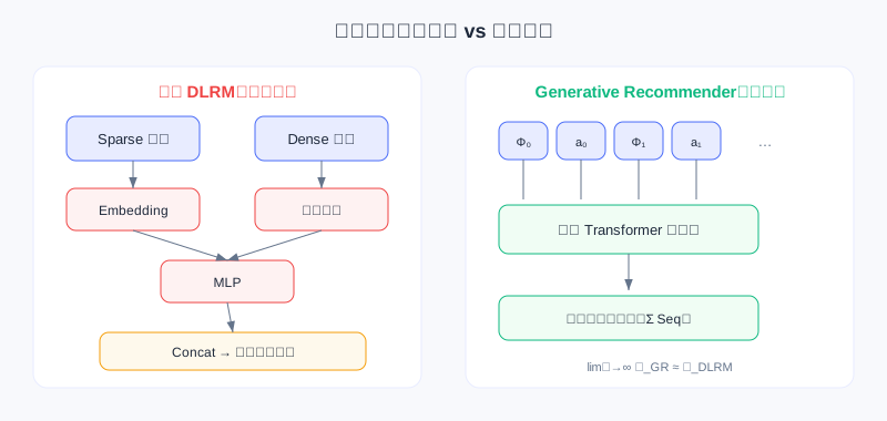
Left: DLRM routes sparse/dense features into different modules, and information stays isolated before concatenation; right: GR encodes all information into a single unified sequence, learned end-to-end by one Transformer.
⚠️ Warning: Fully giving up numerical features is not free. The paper's ablation shows that when the DLRM baseline is also configured as "categorical-only", performance drops significantly. This means in low-compute settings, carefully engineered numerical features still carry value. GR's advantage is learning these signals automatically with larger capacity and longer sequences — a trade of compute for feature engineering.
7.1.3 The Leap in Training Efficiency
The unified sequence representation brings not only modeling advantages — it fundamentally changes the computational complexity of training.
Traditional DLRM: each sample corresponds to one interaction and requires one forward pass. With interactions, you need forward passes, for a total compute cost of .
Under GR, a user sequence has total length . In autoregressive training it provides supervision signals (predict after position 0, predict after position 2, ...). The key point: these predictions are completed in parallel within a single forward pass.
The Transformer's causal mask (lower-triangular mask) ensures position can only see positions through ; one forward pass implicitly encodes all prefixes, and the position after each content token is used to predict the corresponding behavior, all sharing the intermediate results of that same forward pass.
Total compute drops from to — a training efficiency gain of roughly times. With an average of 500 historical interactions per user, that is a 500x speedup. This means with the same compute budget, you can train models one to two orders of magnitude more complex.
💡 Key Insight: This is the first key factor behind GR breaking the scaling bottleneck — it provides enough computational headroom to try deeper networks and larger capacities. But it is not enough on its own; you also need an efficient architecture purpose-built for recommendation.
7.1.4 The HSTU Architecture: A Sequence Model Optimized for Recommendation
Can we just use a standard Transformer? It is proven in NLP, but recommendation has its own peculiarities. Meta's HSTU (Hierarchical Sequential Transduction Unit) introduces three key architectural innovations.
Innovation 1: Pointwise Aggregation Replaces Softmax Attention
Standard Transformer: . Softmax normalization forces attention weights to sum to 1, so what is learned is the relative importance of historical tokens.
But in recommendation we need to know not only "which history matters" but also "how much it matters". For example: user A clicks 10 tech items and 1 entertainment item; user B clicks 100 tech items and 10 entertainment items. Under softmax, both distributions may come out 90%/10% — erasing the information that user B's absolute intensity of interest in tech is higher.
HSTU replaces softmax with pointwise aggregation:
where is the SiLU activation (Swish), is a relative attention bias, and is element-wise multiplication. The full output: , where is a gated projection. The key point is that SiLU maps similarity to a continuous value range but performs no global normalization: each position's weight is independent, and the summed weights can exceed 1 — so the model can learn the absolute intensity of "this user's interest in this type of content is very strong".
Innovation 2: Redesigning Relative Position Encoding
The temporal characteristics of recommendation sequences differ fundamentally from language sequences: language positions are discrete and uniform (words 3 and 5 are always distance 2 apart); recommendation time is continuous and uneven (two interactions may be seconds or months apart).
HSTU introduces an enhanced relative position bias that considers not only the position difference but also the actual time difference , and distinguishes token types (content / action ):
This lets the model learn: recent behaviors matter more, certain behaviors decay faster (browsing vs liking), and the relationship between content tokens and action tokens differs from that between content tokens.
Innovation 3: Simplified Feed-Forward Network and Gating
The standard Transformer appends a two-layer FFN after attention (with the intermediate dimension 4x the hidden size), which consumes most of the parameters and compute. HSTU, inspired by GLU variants, replaces the explicit FFN with element-wise gating:
The gate function is a lightweight transformation. The benefits: (1) it avoids the 4x-hidden FFN, reducing parameters and compute; (2) it cuts activation memory. The latter matters enormously in industry — with very large batch sizes (tens of thousands to hundreds of thousands), activation memory is often the bottleneck. HSTU reduces per-layer activation memory from 33x the hidden dimension in a standard Transformer to 14x, enabling deeper networks under the same memory budget.
📝 Note: The "Hierarchical" in HSTU's name refers to representing ultra-high-cardinality categorical features with hierarchical tokens (e.g., splitting an item ID into multiple sub-tokens). Follow-up research found that a flat representation suffices in most scenarios; the real value lies in the three architectural innovations above.
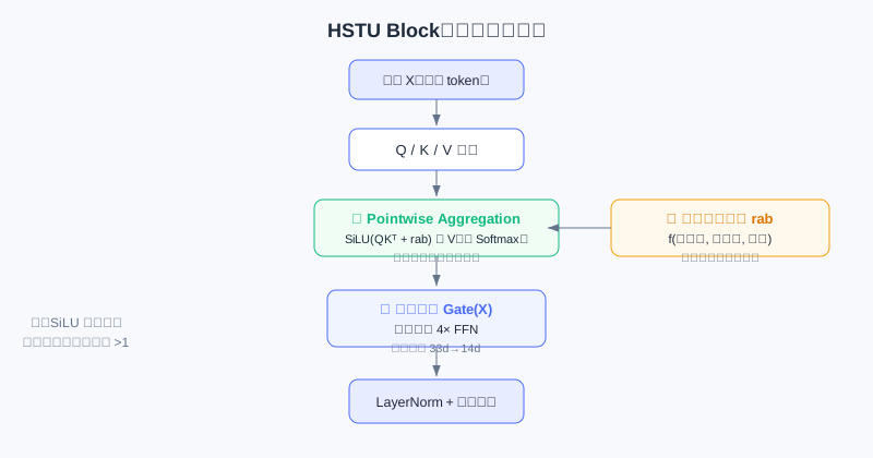
One HSTU Block: after Query/Key/Value projections, element-wise SiLU aggregation (not softmax normalization) with relative time bias is applied, and a gated projection performs the residual fusion.
Analysis: All three HSTU innovations revolve around "the peculiarities of recommendation" — absolute interest intensity (pointwise), non-uniform time (rab), and large-batch memory (gated FFN). Compared with directly applying a standard Transformer, it improves both efficiency and effectiveness, and it is the engineering foundation that makes deploying trillion-parameter models possible.
The interactive demo below lets you see intuitively how HSTU transforms "behavior history" step by step into "behavior prediction": interleaved sequence organization → causal mask → pointwise aggregation → target-aware prediction at candidate positions → multiple supervision signals from one forward pass.
Click "Next" or "Autoplay" and observe how the sequence changes at each step, and why this delivers the leap in training efficiency.
7.1.5 Engineering Optimizations for Training and Inference
With an efficient architecture in hand, ultra-long-sequence training and multi-candidate inference remain hard. HSTU cracks each with an engineering innovation.
Stochastic Length: Exploiting Multi-Scale Redundancy in Behavior
Self-attention complexity is , which becomes unbearable when sequences run to thousands or tens of thousands. But user behavior has repeating patterns at different time scales: long-term stable preferences, mid-term interest evolution, and short-term contextual needs. Based on this observation, HSTU proposes Stochastic Length: for a sequence of length , do not always use the full sequence; instead, with a certain probability randomly truncate to a shorter subsequence.
Concretely, if exceeds a threshold , sample a subsequence of length with probability ; otherwise use the full sequence. controls truncation aggressiveness: smaller (e.g., 1.6–1.7) truncates more aggressively and trains faster; degenerates to no truncation. Subsequence sampling is feature-weighted to ensure coverage across time scales.
This brings a double benefit: (1) self-attention complexity drops from to , sequence sparsity can reach 80%+, and training speeds up several-fold; (2) the random subsequences act as regularization, similar to dropout, forcing the model to learn more robust representations — and generalization actually improves. Experiments show almost no negative impact on quality across a wide range of .
M-FALCON: An Inference Algorithm with Global Cost Amortization
Inference latency is equally critical. Ranking must score hundreds or thousands of candidates one by one; the naive approach needs forward passes with total compute , and the accumulated latency is unacceptable. HSTU's M-FALCON (Microbatched-Fast Attention Leveraging Cacheable OperatioNs) solves it with three escalating optimizations:
Layer 1: Batched Inference — concatenate candidates together and modify the attention mask so candidates cannot see each other (candidate can only attend to the user's history). Now the scores for candidates are computed in parallel in a single forward pass. Setting (full batch), complexity drops to , eliminating the linear dependence on .
Layer 2: Microbatching — when is very large, makes too big. Split the candidates into microbatches (e.g., with on the same order as ) to find the sweet spot between "fully parallel" and "fully serial".
Layer 3: KV Caching — microbatching unlocks KV caching across microbatches: the user-history portion of is identical across all microbatches, so the first microbatch computes the full and subsequent ones only compute the of the new candidates. Later microbatches' complexity drops to , a x speedup. The KV cache can also be reused across requests (the same user refreshing several times within a short window).
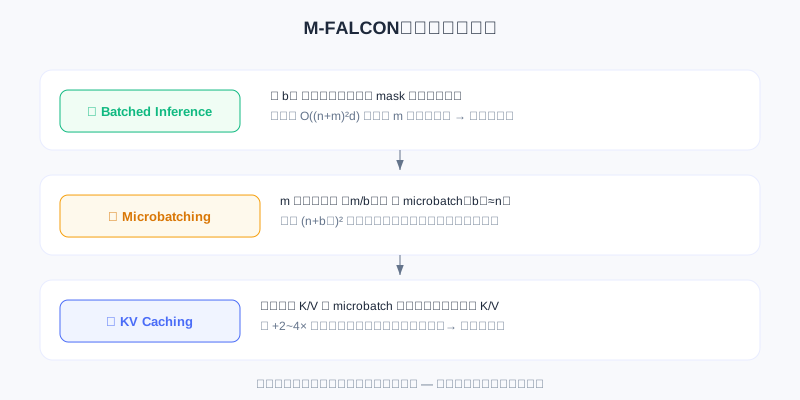
Combined: batched inference brings a tens-of-times speedup, microbatching + KV caching another x — up to hundreds of times overall, letting you use models hundreds of times more complex under the same latency budget.
Analysis: M-FALCON is the engineering cornerstone that lets HSTU deploy trillion-parameter models. It decouples "history representation computation" from the candidate count — the user side is computed only once per request — and this is precisely the origin of the Cross-Request KV Caching idea in OneTrans later in 7.5.
7.1.6 The Scaling Law for Recommender Systems
With all the technical building blocks in place, we return to the original question: can recommendation models keep scaling like language models?
Meta ran systematic scaling experiments: sequence length from 512 to 8192, hidden dimension from 256 to 1024, depth from a few layers to 24. Because recommendation trains in a streaming fashion, training compute was normalized to 365 days to allow fair comparison with GPT-3 and LLaMA-2. Metrics were Hit Rate@100/@500 for retrieval and Normalized Entropy for ranking (lower is better).
Plotted on log axes, all metrics show a clean power-law relationship:
where is the performance metric, is total training compute (PetaFLOPs/day), and are fitted parameters. The fitted results:
- Retrieval:
- Ranking:
That is, for every 10x increase in compute (one order of magnitude), HR@100 improves by about 4.5 percentage points and NE drops by about 1.2 percentage points. More striking still, this relationship holds stably across three orders of magnitude of compute.
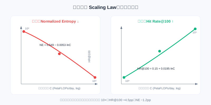
Left: the ranking NE metric keeps decreasing with compute; right: retrieval HR@100 keeps increasing with compute. Both curves are stable across three orders of magnitude, isomorphic to the LLM Scaling Law.
The implications run deep: (1) this is the first proof of a Scaling Law for recommendation models — recommendation is no longer deep learning's exception; (2) small-scale experiments can predict large-scale performance, providing direction for R&D while reducing blind effort and carbon emissions; (3) it opens the door to recommendation Foundation Models — pretrain a large model, then fine-tune across scenarios. The largest configuration (8192 sequence, 1024 dimensions, 24 layers) reached 1.5 trillion parameters and was successfully deployed across multiple Meta surfaces serving billions of users, with online A/B ranking metric gains in the double-digit percentage range.
The interactive curves below let you verify the Scaling Law yourself: drag the slider to adjust training compute and watch Hit Rate@100 and Normalized Entropy move along the power-law curve; you can also click "Next" to walk through several key milestones from small scale to trillion-parameter deployment.
Each 10x increase in compute moves HR@100 up about +4.5pp and NE down about −1.2pp — this predictability is the fundamental guarantee that recommendation models can scale like LLMs.
7.1.7 Why Could HSTU Break Through?
Looking back at the whole technical system, four levels of innovation support one another:
- The paradigm shift is the foundation — moving from item-level to user-level, from independent scoring to sequence generation, unbinding compute cost from candidate count's linear coupling.
- Architectural innovation is the key — attention, position encoding, and the feed-forward network were each purposefully designed, yielding significant gains over directly applying a standard Transformer.
- Engineering optimization is the guarantee — Stochastic Length makes ultra-long-sequence training feasible, M-FALCON makes complex-model inference efficient, and activation memory optimization makes large batches a non-issue.
- The unified feature space is the base — heterogeneous features enter a unified sequence, simplifying feature engineering and, more importantly, letting the model learn complex interactions end-to-end with higher parameter efficiency.
All four are indispensable. HSTU's success proved recommendation models can scale — and left new questions behind: which factors are truly essential? Is fully generative training necessary? How do we generalize to multi-task, multi-surface settings? Later research answers these — starting with GenRank in 7.2, which asks "is the autoregressive mechanism really the essence?"
⚠️ Common Mistakes in 7.1
| # | Mistake | Example | Why It's Wrong | Fix |
|---|---|---|---|---|
| 1 | Assuming recommendation inherently cannot scale | "Adding parameters to a DLRM is useless; recommendation is just the exception" | It is not that recommendation cannot scale; the item-level paradigm + fragmented architecture tie its hands computationally | Understand how HSTU's user-level sequences unbind it |
| 2 | Treating GR as ordinary sequential recommendation | "GR is just SASRec with longer sequences" | GR models content–action interleaved sequences and predicts behaviors in a target-aware way | Distinguish item sequences from behavior sequences |
| 3 | Assuming softmax attention is good enough | "Just use a standard Transformer as HSTU" | Softmax normalization erases the absolute intensity of interest | Remember the key difference of pointwise aggregation |
| 4 | Overlooking where the training efficiency comes from | "Sequence modeling just performs better" | One forward pass yields supervision signals, speeding training up times | Understand the compute dividend of user-level aggregation |
| 5 | Assuming the Scaling Law only holds for huge models | "Scaling only matters at a trillion parameters" | The power law holds across three orders of magnitude; small-scale experiments extrapolate | Use small experiments to predict large-scale performance |
Chapter Summary
📌 Key Takeaways
| Concept | Key Points | Why It Matters |
|---|---|---|
| Three DLRM limitations | Feature bottleneck / architectural fragmentation / item-level training | Explains why recommendation long failed to scale |
| GR paradigm | interleaved sequence, user-level autoregression | Unified sequence + multiple supervision signals, x training speedup |
| Three HSTU innovations | Pointwise Agg / relative time bias / gated FFN | A sequence architecture tailored to recommendation |
| Stochastic Length | Random truncation of ultra-long sequences | Several-fold training speedup + regularization |
| M-FALCON | Batched→Microbatch→KV Cache | Hundreds-of-times inference speedup, trillion parameters deployable |
| Scaling Law | , stable across three orders of magnitude | First proof recommendation can scale; opens the door to foundation models |
❓ FAQ
Q1: Why is Pointwise Aggregation better suited to recommendation than Softmax?
A: Softmax forces weights to sum to 1 and learns only "relative importance"; recommendation also needs "absolute intensity" (user B likes tech more than user A does). SiLU element-wise aggregation does no global normalization, weights can accumulate beyond 1, and absolute interest intensity is preserved — which is crucial for predicting post-click deep behaviors.
Q2: Why is GR training so much faster than DLRM?
A: A DLRM does one forward pass per interaction — samples means forward passes. GR predicts behaviors for a user sequence in one forward pass (sharing computation under the causal mask), so total forward passes drop to , roughly an x speedup.
Q3: Why are recommendation foundation models now plausible?
A: The Scaling Law proves performance improves predictably with compute, which means you can pretrain a large general recommendation model and fine-tune it across scenarios — the most exciting direction after HSTU's 1.5-trillion-parameter deployment.
🔗 Connections to Later Chapters
- 7.2 (Generative Ranking / GenRank) asks whether autoregression is the essence and speeds things up further with Action-Oriented design — directly continuing this chapter's question of "which factors are essential".
- 7.3 (MTGR) retains cross features under a hybrid paradigm, answering "is fully generative training necessary?"
- 6.1–6.4 (generative fundamentals) provide the prerequisites of semantic IDs and RQ-VAE for understanding how items become tokens.
- 3.1–3.5 (discriminative ranking) are the "old paradigm" this chapter keeps contrasting against — see the bottlenecks clearly, and the breakthrough lands.
Practice Problems
Work through all problems in order — they get progressively harder. Each has a complete solution you can reveal after trying it yourself.
Problem 7.1.1 — Identifying the DLRM Bottleneck 🟢 Easy
A team doubles the DLRM's embedding dimension and deepens the MLP, yet online CTR-prediction AUC barely moves. Based on the three limitations in 7.1.0, identify the most likely cause (pick one and justify it).
💡 Solution (click to reveal)
Approach: Judge from the angle of "more capacity ≠ more information".
The most likely culprit is the feature bottleneck: the DLRM compresses history into pre-aggregated numerical features (CTR, average watch time), so model capacity grew but the richness of input information did not. Second is item-level training — each sample carries only one supervision signal, so added capacity does not increase the per-sample information. Architectural fragmentation is also possible (scaling one module only improves things locally).
Key points:
- A stalled compute growth curve usually means information or the paradigm is constrained, not that parameters are insufficient.
- This is precisely what leads to HSTU's user-level sequence solution.
Problem 7.1.2 — GR Sequence Organization 🟢 Easy
Traditional sequential recommendation models the item sequence , while HSTU's GR models . Answer:
- How many times the number of interactions is the GR sequence length (in tokens)?
- Is the ranking task target-aware or target-agnostic?
💡 Solution (click to reveal)
Approach: Map directly to the definitions in the text.
- The GR sequence has total length (content and action alternating), which is 2 times .
- In the model sees candidate before predicting behavior , so it is target-aware.
Key points:
- The interleaved sequence trades length for behavioral feedback signals.
- Target-awareness is the foundation for later generative ranking to predict deep behaviors.
Problem 7.1.3 — Training Efficiency Multiple 🟡 Medium
Suppose users average historical interactions and the training set has interaction records. Compare the order of magnitude of "forward passes" required by the DLRM (one per record) versus GR (organized into user sequences of length ). About how many times faster is GR?
💡 Solution (click to reveal)
Approach: DLRM forward passes = . GR organizes the interactions into sequences, one forward pass each.
forward passes. The speedup is x.
Key points:
- The speedup ratio ≈ average sequence length , because one forward pass yields supervision signals.
- This explains "with the same compute you can train models hundreds of times more complex".
Problem 7.1.4 — Extrapolating the Scaling Law 🔴 Hard
Given retrieval HR@100 ( in PetaFLOPs/day). If compute grows from to (one order of magnitude), by how many percentage points does HR@100 improve? And why is this more controllable than "blindly stacking parameters"?
💡 Solution (click to reveal)
Approach: Use the difference of logarithms.
. That is about 4.5 percentage points, consistent with the main text.
Key points:
- The Scaling Law gives a predictable power law, so small experiments can extrapolate to large-model performance.
- Compared with blindly stacking parameters (which may plateau), it turns R&D into a controlled engineering exercise of "planning performance against the compute budget".
🏆 Challenge: Arguing a Design Trade-off
Suppose you lead a mid-sized company's recommendation team with only 1% of Meta's compute. Write an argument within 150 words: should you copy HSTU's trillion-parameter setup directly, or first do a lightweight landing based on its "paradigm shift + engineering optimization" ideas? Identify the two HSTU techniques most useful to you.
💡 Hint
With limited compute, a trillion parameters is infeasible; but "user-level sequence training's x speedup" and "M-FALCON's KV caching/batching" are architecture dividends independent of compute scale, and the most worth borrowing. Stochastic Length's truncation also directly cuts training cost. The point is to carry over the paradigm dividend, not the parameter scale.
The Overall Generative Ranking Paradigm
📝 Before You Continue: Make sure you have finished 7.1 HSTU. This chapter traces HSTU back to its roots — it repeatedly returns to HSTU's design decisions and asks which are essential and which can be optimized. Understanding 7.1's architecture and engineering is what makes GenRank's trade-off logic click.
HSTU proved with a trillion-parameter model that recommendation can follow the Scaling Law — but on top of Meta's gigantic compute: a trillion parameters, thousands of GPUs, and billions of users' data every day. For the vast majority of companies, that bar is far too high.
This raises a key question: in HSTU's design, which parts are essential, and which can be optimized? The Xiaohongshu team faced this challenge in practice — they wanted to bring generative recommendation to a system serving hundreds of millions of users, and first had to answer: where exactly does the effectiveness of generative recommendation come from?
7.2.0 Tracing It Back: What Is the Essence?
To optimize HSTU, first understand where its effectiveness comes from. HSTU is a complex system: generative architecture, autoregressive training, sequential organization, and a unified feature space all act together. But engineering demands clarity on each factor's true contribution — if some design contributes only 0.1% performance while costing 10x overhead, it should be dropped when resources are constrained.
The Xiaohongshu team ran controlled experiments on hundreds of billions of real exposure logs, using HSTU as the baseline and changing one design decision at a time. The first thing to verify: is the autoregressive mechanism necessary?
Recall HSTU: it trains with a causal mask but computes loss only at candidate item positions — history positions contribute nothing, similar to LLM SFT (user history + candidate form the prompt, and the model predicts the behavioral feedback). In LLMs, SFT stays autoregressive to preserve pretrained capability; but recommendation usually has no pretraining stage — could autoregression be just an optional trick?
Two controlled experiments:
First group: also compute loss at history positions. If autoregression were just an optional trick, more supervision signals should improve performance — but AUC drops significantly. This can be explained by the "one-epoch problem": sparse features like user/item IDs account for the vast majority of parameters, and under long-tail distributions huge numbers of IDs appear only once or twice. Computing loss at history positions pushes the model to "memorize" every interaction detail while failing to generalize (e.g., the user's history says "watched tech A → liked"; at test time the user watches tech C, a combination the model has never seen). And recommendation usually trains for only one epoch, leaving no chance to correct this overfitting.
Second group: use a fully-visible mask at history positions (bidirectional attention). From a feature-interaction standpoint this should strengthen expressiveness, yet performance still drops — and the drop widens as the model grows. The fully-visible mask destroys a key inductive bias — the causality of user interest evolution. The causal mask forces learning of causal structure rather than arbitrary statistical correlation. For example, if bidirectional attention is allowed, when processing "watched tech A" the model can also see the later "liked" and "watched food B", and may learn a spurious association ("liked the tech video because food came after") — but in reality, behavior at time cannot be influenced by the future.
Both experiments point to the same conclusion: the autoregressive mechanism is the essential characteristic of generative recommendation. Through an architectural constraint it introduces a beneficial inductive bias, helping the model learn the causal structure of behavior while curbing overfitting to sparse features.
🧠 Mental Model: Autoregression as "Causal Glasses"
Think of the causal mask as putting a pair of causal glasses on the model: it can only look forward, forcing it to learn "how the past led to the present". Take the glasses off (bidirectional attention) and the model peeks at answers and learns spurious associations. These glasses are not a performance burden but regularization against cheating — this is where autoregression's essential status comes from.
Sample organization, by contrast, matters much less. The traditional DLRM trains point-wise (one interaction per sample); HSTU organizes user-level into sequences. But experiments show: keeping the sequential organization while computing loss only at the last position (mimicking point-wise) barely hurts performance. This means user-level organization mainly brings engineering convenience (high throughput, easy KV caching), not a fundamental source of performance.
The team also tested compatibility with commonly used industrial modules: SIM, PPNet, and PLE remain effective under a generative architecture; most historical aggregate features lose most of their value (sequence modeling learns the statistical patterns automatically), but real-time features remain important (capturing new information outside the training window). Simplified feature engineering also freed system resources, making room for handling larger candidate sets.
7.2.1 Action-Oriented: Re-understanding the Task's Essence
HSTU's core is the interleaving formula: , modeled as a Markov chain. But analyzing the computational cost reveals a problem: with user interactions + candidates, the sequence is length and attention complexity is . When reaches thousands, is a heavy burden.
The core question: given the user's history and candidates, what do we actually need to predict? The answer is what behavioral feedback the user will produce on an item (click rate, watch time, like probability). In ranking, the item is given context and the behavior is the prediction target — the item is more like context or a positional identifier.
Take Xiaohongshu ranking 100 candidates as an example: for each note, predict "will they click / how long will they watch / will they like". The note itself (title, images, author) is a known input; behavioral feedback is the output. Given that, is it necessary to treat "note" and "behavior" as equals (each occupying a token position)?
Based on this, GenRank evolves: make behaviors the sequence's main body and items the attributes of behaviors:
where denotes "the behavior the user produced on item " — this is Action-Oriented Organization.
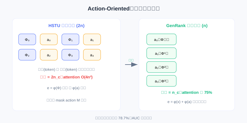
Top: HSTU's interleaved sequence spends 2 tokens per interaction; bottom: GenRank fuses the item into the same token as an attribute of the behavior, cutting sequence length from to .
Technically, each token is represented as:
Item embedding and behavior embedding fuse directly in the same space; candidate items use a special mask for the action embedding: .
The immediate benefit: sequence length halves (from to ), which cuts attention compute by 75%, linear projections by 50%, activation memory by about 50%, and the KV cache in half. Experiments show this change alone brings a 78.7% training speedup.
Does this lose information? From an information-theoretic view, user behavior is strongly influenced by item content — the two have high mutual information. Addition lets the embeddings "align" in representation space: important dimensions reinforce their signals, unique dimensions preserve their information. For example, if some dimension encodes "entertainment value", a funny video's item embedding might be 0.8 and the "like" behavior embedding 0.6, summing to 1.4 with the signal amplified; a dimension encoding "video duration" relates only to the item, the behavior embedding is near 0, and the item information is preserved; "completion rate" relates only to the behavior, and the behavior information is preserved. Since item/action tokens interact most frequently within HSTU's attention anyway, fusing them at the token level actually lightens the attention layer's load.
Action-oriented also enables a more flexible mask: scoring a batch of candidates has two conflicting requirements — candidate scores must be independent (in real exposure, the user sees one item at a time), yet all candidates must see the full history. GenRank balances this with a specific mask: causal mask among history tokens; candidates can attend to all history but are masked from each other. This guarantees independence while leaving room for a future extension to sequential re-ranking.
7.2.2 Position and Time: What to Learn and What to Encode
Action-oriented solves sequence length, but another bottleneck remains: encoding position and time information.
HSTU uses a relative attention bias (RAB):
Considering position difference, time difference, and even token type lets the model learn patterns such as temporal decay. The problem is that compute/memory overhead is : for a sequence of length , is an matrix that must be read in the forward pass and differentiated in the backward pass. When reaches thousands, runs to millions; in modern training, memory bandwidth is the bottleneck, and memory access burns time on data movement, degrading GPU utilization.
GenRank's alternative: encode absolute information with lightweight embeddings and relative information with parameter-free biases.
The core idea: position/time decomposes into two parts — absolute information ("which interaction", "when it happened") uses embeddings; relative information ("how far apart two interactions are") uses a simple parameter-free rule. GenRank uses three lightweight embeddings:
- Position Embeddings: , recording the sequence index; candidates within a request share the position index, keeping training/inference consistent.
- Request Index Embeddings: , capturing behavioral burst patterns (users often open the app once, interact several times in a row, then leave; this helps the model distinguish within-session from cross-session interests).
- Pre-Request Time Embeddings: , encoding the gap since the last request, achieving adaptive decay (for high-frequency users a short gap is meaningful; for low-frequency users a few hours is nothing).
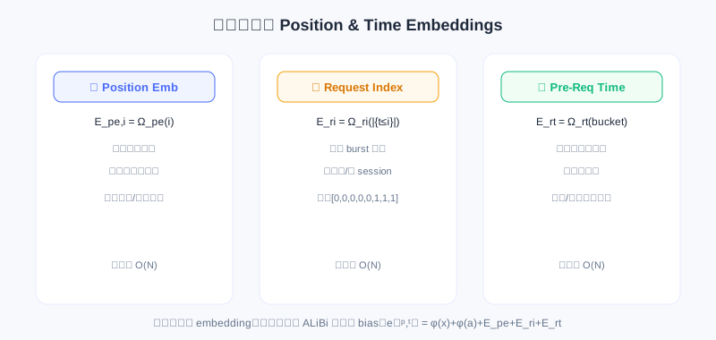
The three embeddings are added to the token representation: . Total parameters are only a few million, with I/O complexity.
For relative information, GenRank borrows from ALiBi (Attention with Linear Biases): apply a penalty proportional to distance to distant query-key pairs:
ALiBi's three advantages: it matches intuition (farther means less influence), it has no parameters ( is predefined), and it can be fused into the FlashAttention kernel. GenRank extends it to consider both position and time:
🧠 Mental Model: Parameters vs Rules
Think of the encoding strategy as a division of labor: complex, non-linear patterns (like "which interaction" or "which app open") go to learnable embeddings; universal, approximately linear rules (like "farther means less important") are written directly as rules. It is like a company — oddball cases go to specialists, standard workflows become SOPs that run automatically, and not everything needs a meeting.
History tokens use a causal mask (lower-left triangle visible); candidates can attend to all history; candidates are masked along the diagonal (mutually independent).
Experiments show: action-oriented alone gives a 78.7% speedup, and the new position & time biases add another 25.0% — 94.8% total speedup, with AUC slightly up. A simpler design achieves better results, validating the principle: good inductive biases matter more than raw parameter capacity.
💡 Key Insight: Going from HSTU to GenRank marks recommendation's shift from "engineering-driven" to "principle-driven". The autoregressive mechanism is the core; training paradigm details can be optimized flexibly. But GenRank keeps the purity of the generative formulation — which means giving up the cross features of traditional DLRMs that need to observe historical statistics and candidate attributes simultaneously. This leads to 7.3's soul-searching question: must the efficiency advantage of user-granularity modeling be bound to the fully generative formulation?
⚠️ Common Mistakes in 7.2
| # | Mistake | Example | Why It's Wrong | Fix |
|---|---|---|---|---|
| 1 | Treating autoregression as just a training trick | "Removing the causal mask and adding bidirectional attention should be stronger" | It destroys the causal inductive bias, learns spurious associations, and AUC drops | Remember autoregression is the essential feature of generative models |
| 2 | Treating user-level organization as the source of performance | "Aggregating sequences by user is what makes HSTU strong" | Experiments: loss only at the last position (mimicking point-wise) barely hurts performance | It mainly brings engineering convenience (throughput/KV cache) |
| 3 | Assuming Action-Oriented loses information | "Fusing item and behavior into one token must lose something" | Their mutual information is high; addition reinforces aligned dimensions and preserves unique ones | Understand that token-level fusion actually reduces load |
| 4 | Dismissing RAB's | "Just learn the relative position bias directly" | At thousands of length, becomes a memory-bandwidth bottleneck and GPU utilization drops | Use lightweight embeddings + parameter-free ALiBi bias |
| 5 | Mixing absolute/relative encodings | "Encode all time information with learnable matrices" | Universal rules need not be learned; overparameterization invites overfitting | Complex patterns via embedding, linear rules via rules |
Chapter Summary
📌 Key Takeaways
| Concept | Key Points | Why It Matters |
|---|---|---|
| Autoregression is the essence | Two controlled experiments prove the causal inductive bias cannot be dropped | The dividing line between "means" and "ends" |
| User-level organization | Mainly engineering convenience, not a performance source | Can be adjusted flexibly without hurting the essence |
| Action-Oriented | Behaviors as main body, items as attributes; sequence halved | 78.7% training speedup with almost no performance loss |
| Lightweight position/time encoding | 3 embeddings + parameter-free ALiBi bias | Another 25% speedup, 94.8% total |
| Inductive bias > parameter capacity | A simpler design performs better | Guides optimization under constrained resources |
❓ FAQ
Q1: Why can't autoregression be removed in favor of bidirectional attention?
A: Bidirectional attention lets the model peek at "future" behaviors, learns spurious statistical associations, and destroys the causal structure of user interest evolution; the performance drop widens as the model grows. The autoregressive causal mask is beneficial regularization against overfitting sparse features.
Q2: With Action-Oriented fusing items into behavior tokens, can ranking still distinguish different candidates?
A: Yes. Each candidate has an independent token , and item information distinguishes them via ; the between-candidate mask keeps them mutually blocked, guaranteeing independent scores. Halving the sequence only reduces positions; it does not conflate candidate identities.
Q3: Why use ALiBi for relative-distance decay instead of learning it?
A: "Farther means less important" is a universal, approximately linear rule — encoding it directly is more efficient and stable, and it fuses into the FlashAttention kernel; overparameterizing it reduces training efficiency and adds overfitting risk. Complex non-linear patterns are what deserve learnable embeddings.
🔗 Connections to Later Chapters
- 7.1 (HSTU) — all the "root tracing" in this chapter builds on its architecture/engineering, directly answering "which factors are essential".
- 7.3 (MTGR) picks up the closing soul-searching question: is the efficiency advantage necessarily bound to the fully generative formulation? MTGR answers no with a hybrid paradigm.
- 3.4 (Multi-objective/MMoE) — the text mentions PLE remains compatible under a generative architecture, a continuation of discriminative multi-objective modules.
Practice Problems
Work through all problems in order — they get progressively harder. Each has a complete solution you can reveal after trying it yourself.
Problem 7.2.1 — Judging the Necessity of Autoregression 🟢 Easy
Which of the following two changes is expected to improve performance, and which to hurt it? Explain why.
- (a) Also computing loss at history positions (more supervision signals)
- (b) Keeping user-level sequences but computing loss only at the final candidate position
💡 Solution (click to reveal)
Approach: Map to the two experiments in the text.
- (a) Hurts: loss at history positions pushes the model to memorize details and hurts generalization (one-epoch overfitting); AUC drops significantly.
- (b) Almost unchanged: this is exactly what GenRank verified — user-level organization mainly brings engineering convenience, not performance.
Key points:
- Autoregression (causal) is the essence; adding bidirectional supervision actually hurts.
- Organization is flexible; the architectural constraint is the core.
Problem 7.2.2 — Action-Oriented Sequence Length 🟢 Easy
For HSTU's interleaved sequence with historical interactions, how many tokens is the sequence? Under GenRank's Action-Oriented, how many? By what factor does attention compute (proportional to length squared) drop?
💡 Solution (click to reveal)
Approach: Apply the formulas directly.
- HSTU: tokens.
- GenRank: tokens (behaviors as main body, items fused as attributes).
- Attention compute scales with length squared: , i.e., a 75% reduction.
Key points:
- Halving the sequence → a quadratic drop in compute.
- This matches the text's "attention reduced by 75%".
Problem 7.2.3 — Division of Labor in Encoding 🟡 Medium
How does GenRank encode "which app open this is for the user (request index)" and "how far apart two interactions are (relative time)" respectively? Why this division of labor?
💡 Solution (click to reveal)
Approach: Distinguish absolute vs relative information.
- Request index (which open) = absolute, structured, different positions carry different semantics → use a learnable Request Index Embedding .
- Relative time decay (farther means less important) = a universal, approximately linear rule → use a parameter-free ALiBi bias .
Key points:
- Principle: parameters for complex non-linear patterns, rules for universal linear ones.
- Avoid the overfitting and memory bottleneck of overparameterization.
Problem 7.2.4 — Attributing the Speedup 🔴 Hard
A team reproduces GenRank: Action-Oriented alone gives a 78.7% speedup, and adding the new position/time encoding gives a 94.8% total speedup. How much extra speedup does the new encoding contribute relative to the "already Action-Oriented baseline"? (Hint: a 78.7% speedup means time drops to 21.3%.)
💡 Solution (click to reveal)
Approach: Multiply the time ratios.
After Action-Oriented, time = . After the total 94.8% speedup, time = . The speedup ratio of the new encoding relative to the Action-Oriented baseline is , i.e., roughly an extra 75.6% speedup (equivalently, the new encoding cuts time further to ).
Key points:
- Speedups compose multiplicatively, not additively.
- This also confirms "lightweight encoding" saves another 25% of total time on top of Action-Oriented.
🏆 Challenge: Arguing a Design Optimization
You need to deploy generative ranking under limited compute. Within 150 words, argue: which two designs from HSTU/GenRank should you prioritize keeping, and which kind of feature engineering can you drop? Tie your argument to "autoregression is the essence" and "real-time features still matter".
💡 Hint
Must keep: (1) the autoregressive causal mask (the essence, providing the causal inductive bias); (2) user-level sequence organization + Action-Oriented (engineering dividend, nearly 80% training speedup). Droppable: most historical aggregate features (sequence modeling learns them automatically), but keep real-time features (new information outside the training window). This echoes 7.2's experimental conclusions.
MTGR: Hybrid Paradigm Modeling
📝 Before You Continue: You have read 7.2 Generative Ranking. This chapter picks up its closing soul-searching question — is the efficiency advantage of user-granularity modeling necessarily bound to the fully generative formulation? MTGR answers no with a "hybrid paradigm".
HSTU proved recommendation can follow the Scaling Law, and GenRank revealed that the essence of generative modeling is autoregression rather than the training paradigm. Both evolved toward "purity": unified sequence modeling replaces fragmented feature engineering, and an end-to-end Transformer replaces heterogeneous modules.
But this purity has a price.
In HSTU/GenRank, to achieve full behavior-sequence modeling, predicting user behavior on a candidate cannot use any candidate-dependent cross features. These are hard-won lessons from years of industry iteration — "the user's historical CTR on this category", "the user's preference for this kind of content at this hour", "how well the item matches the user's profile" — precisely capturing fine-grained user-candidate interactions.
The Meituan team discovered a stark fact: removing cross features causes a significant performance drop, and even substantially increasing model scale cannot make up for it. This raises the fundamental question: can the user-granularity modeling paradigm of generative recommendation be combined with the feature engineering experience of traditional DLRMs?
MTGR (Meituan Generative Recommendation) answers yes. Its core contribution is not faster training or lower latency, but a hybrid paradigm: retaining the efficiency of user-granularity aggregation while supporting target-aware discriminative modeling.
7.3.0 Rethinking the Paradigm: Generative vs Discriminative
The Fundamental Assumption of HSTU/GenRank
Both adopt interleaved modeling , with the joint distribution decomposed as . The ranking task corresponds to — which looks target-aware, because the model sees the candidate .
The problem is: the candidate is part of the sequence, on equal footing with the historical behavior . Under autoregressive training, the prediction at position can only depend on positions through . But cross features often need to "cross over" this ordering — they require simultaneously looking at some historical statistic of the user (e.g., "average dwell time on tech content") and the current candidate's attributes ("this is a tech video") before computing the interaction. Under a purely generative scheme this crossing is forbidden: if 's representation were allowed to depend on "the user's historical preference for this candidate's category", causality would break — because that feature has effectively "seen the future" (it was computed against the current candidate ).
GenRank's action-oriented compresses sequence length but does not change this fundamental restriction; strict temporal ordering is still preserved.
Meituan's ablation gives a clear answer: after removing cross features, even the largest-scale generative model degrades to worse than a mid-scale traditional DLRM. This is a gap scaling cannot fill — it is missing information, not missing capacity.
The Essence of Discriminative Ranking
Why are cross features so critical? Look at the nature of the ranking task: the input is the user's history plus a set of candidates, and the task is to predict a behavioral propensity (click, dwell, conversion) for each candidate. This is a classic discriminative task: given input (history + candidate), predict label (behavior).
The traditional DLRM formulates it as , where is the user representation and is the item representation. The key point: the user representation may depend on the candidate item . For example, "the user's average CTR on tech content" is only meaningful when the candidate is a tech item — this is a interaction, second-order or even higher. Many important signals come from "conditional statistics" (the user's historical behavior on this kind of content at this hour, this creator's content's appeal to this kind of user), which require simultaneously observing a subset of user history and candidate attributes before computing the statistic — hard to express naturally in a generative fashion.
Probabilistically, the discriminative approach cares about the conditional distribution and need not model the full joint . The generative approach derives the conditional from a factorized joint, at extra cost: it must model — even when that is not what we actually care about.
MTGR's Core Insight
The efficiency gain of user-granularity modeling comes essentially from sample aggregation and computation reuse — it does not require full generative modeling.
7.3.1 MTGR's Hybrid Paradigm
MTGR proposes a scheme that sounds contradictory but is in fact clever: use the architecture of a generative model (Transformer + user-granularity aggregation) while keeping a discriminative modeling objective.
Concretely, the data organization aggregates multiple candidates of the same user into one sample:
The key differences:
- The history part (User, Seq, RealTime) matches HSTU/GenRank — the user's full behavior sequence
- The candidate part (Cross, Item) is no longer a continuation of history but the prediction target; each candidate's representation directly contains cross features
This breaks the strict "content–action alternating" temporal structure, admitting: at the ranking stage, candidates are given inputs, not intermediate states to be generated. Therefore targeted features can be constructed for each candidate (including cross features that depend on historical statistics and candidate attributes).
User/sequence/real-time tokens encode the history; multiple candidate tokens each fuse item features and cross features (such as ctr, pv) and are processed in parallel. Including cross features in the candidate part is MTGR's key advantage over pure generative approaches.
Meaning of each token: User tokens (static attributes like age, gender, city); Sequence tokens (long-term behavior sequence); RealTime tokens (recent interactions); Candidate tokens (one per candidate, fusing item + cross features).
This organization retains the user-granularity aggregation advantage: for candidates, the history part (User+Seq+RealTime) is encoded only once, with the candidate tokens in parallel. Complexity is rather than — a significant speedup when . But MTGR no longer models the full behavior sequence; it computes loss and predicts behavior only at candidate positions — the discriminative objective allows candidate representations to contain arbitrary user-item cross information.
💡 Key Insight: MTGR's philosophy is separating means from ends. The generative architecture (Transformer + sequence modeling) is a powerful representational means, but it need not serve a generative objective; user-granularity aggregation is an efficient computational organization, but it need not require a fully causal sequence. The hybrid paradigm retains efficiency while restoring the flexibility of discriminative modeling.
7.3.2 Architectural Innovation 1: Mapping Features to Tokens
Problems appear when introducing cross features into a unified framework. Consider 3 candidates:
- Candidate 1: tech video; the user's historical CTR on tech is 0.8
- Candidate 2: food video; the user's historical CTR on food is 0.3
- Candidate 3: tech video; the user's historical CTR on tech is 0.8
Candidates 1 and 3 share identical cross features but are distinct candidates that should be scored independently. MTGR constructs an independent token for each candidate, fusing:
- The item's intrinsic features (ID, category, tags, duration)
- Cross features (the user's historical CTR on this category, preference at this hour)
- Position and temporal information (list position, exposure time)
Formally, for candidate :
The key decision: cross features are treated as part of the candidate representation, not as part of the history sequence. Even though candidates 1 and 3 share the same cross features, two independent tokens are still generated (because other dimensions like item ID and title differ).
Token generation for the user-history part is straightforward: User tokens (one per attribute), Sequence tokens (one per historical item), RealTime tokens (one per recent interaction) — all "pure", depending on no candidate, encoding only history.
This asymmetric token organization creates a problem: different token types live in different semantic spaces. User tokens encode demographics, Sequence tokens encode behavior patterns, Candidate tokens encode item + cross features. Processing them directly with a unified Transformer makes tokens from different semantic spaces interfere with one another.
7.3.3 Architectural Innovation 2: Group Layer Normalization
Standard LayerNorm normalizes along the token's feature dimension: , assuming all tokens share the same feature distribution with global parameters .
Under MTGR this assumption breaks. Consider a batch's token sequence:
An Age token's activations may lie in (discrete demographics), while Sequence tokens may span (accumulated over more layers). Global LayerNorm computes mean and variance across all tokens, leaving Age "over-amplified" and Sequence "over-compressed". Worse is semantic confusion: dimension 100 may encode "user activity level" in a User token but "candidate popularity" in a Candidate token; global normalization mixes them together and weakens representation.
MTGR proposes Group Layer Normalization (GLN): normalize in groups by token type.
- Group 1: User tokens
- Group 2: Sequence tokens
- Group 3: RealTime tokens
- Group 4: Candidate tokens
Within each group, mean, variance, and normalization parameters are computed independently:
where is the group of token .
Left: standard global LayerNorm mixes all tokens together, with distributions and semantics interfering; right: GLN normalizes the User/Seq/RT/Cand groups independently, aligning distributions and keeping semantics separate.
The benefits: (1) distribution alignment — tokens within a group are semantically close with similar distributions, so independent normalization stabilizes training; (2) semantic independence — the same dimension can encode different information in different groups, and parameter independence guarantees semantic independence. GLN merely adds group information to LayerNorm, with negligible computational overhead — yet it acknowledges an important fact: in a hybrid paradigm, different types of information should stay relatively independent in representation space rather than being forcibly unified. This principle appears elsewhere in MTGR too (different groups can use embeddings of different dimensions, different layers for processing) — it is the balance point between unified architecture and feature flexibility.
7.3.4 Architectural Innovation 3: Dynamic Masking
Transformer self-attention allows arbitrary token interaction, but sequence modeling usually requires restrictions for causality. HSTU/GenRank use a causal mask (lower triangle). But under MTGR's hybrid paradigm the causal mask no longer applies — the token sequence is not organized strictly by time.
Recall MTGR's organization: . User is static, Seq is already time-ordered, RealTime is recent (and may overlap the candidates' exposure times), Candidates are parallel (and should not see each other, since in real exposure the user views one item at a time). A naive causal mask runs into problems: Cand would see Cand, but in training the candidates were exposed at different times and at inference they must be scored simultaneously — visibility between candidates makes no sense.
The thornier issue is handling RealTime. RealTime records interactions in a recent window (say, the last hour). If multiple exposures across a day are aggregated, RealTime may contain interactions that happened after some candidate's exposure — causing information leakage. For example: 12:00 sees candidate A (clicked), 12:30 sees candidate B (not clicked), 13:00 sees candidate C (clicked). In aggregated training, RealTime contains the 13:00 click, but when predicting candidate B at 12:30 the model should not see it.
MTGR's Dynamic Masking solves this with fine-grained visibility control, defined by three rules:
Rule 1: Static sequences are visible to all tokens — User and Seq come from history before the aggregation window, and any candidate may attend to them (long-term history is meaningful for all candidates). In the mask matrix, the User/Seq columns are all 1s.
Rule 2: Dynamic sequences follow causality — RealTime tokens' timestamps may fall inside the aggregation window, ordered relative to candidate exposures. RT's visibility to RT depends on timestamps ( means visible); RT's visibility to Cand also follows timestamps (visible if Cand's exposure time). In the mask, RealTime is causal among itself (lower triangle), and toward Candidates it is decided dynamically by actual timestamps.
Rule 3: Candidates are mutually independent — Cand is invisible to Cand (), guaranteeing independent scores. In the mask, the Candidate blocks form a diagonal mask (only the diagonal is 1).
White means visible, gray invisible: the user-feature and history-sequence columns are fully white (globally visible); the real-time sequence is partially triangular by timestamp (causal); candidates are visible only on the diagonal (independent).
This mask is not fixed in advance but generated dynamically from the actual timestamps of each sample's tokens — hence the name "Dynamic Masking". It prevents information leakage: in training it stops the model from learning spurious causality; at inference it lets all candidates of a request be processed in parallel (RealTime contains only pre-request interactions, and candidates are mutually independent), preserving computational efficiency. Dynamic Masking is the final piece of the hybrid paradigm, letting one Transformer handle both causal sequences (history) and non-causal targets (candidate scoring), striking the balance between flexibility and correctness.
Analysis: MTGR does not chase the fastest training but compatibility — using the generative architecture's computation reuse (user-level aggregation, ) to buy back the discriminative flexibility of cross features. GLN and Dynamic Masking are the two key techniques that let heterogeneous tokens coexist in one Transformer: the former resolves semantic-space conflicts, the latter temporal/independence conflicts.
⚠️ Common Mistakes in 7.3
| # | Mistake | Example | Why It's Wrong | Fix |
|---|---|---|---|---|
| 1 | Assuming scale can compensate for cross features | "Remove cross features and scale up the model to make it up" | Meituan's experiments: the largest generative model still loses to a mid-size DLRM | Cross features are missing information, not missing capacity |
| 2 | Treating MTGR as purely generative | "MTGR is just HSTU plus features" | MTGR computes loss only at candidate positions — a discriminative objective | It is a hybrid paradigm: generative architecture + discriminative objective |
| 3 | Stuffing cross features into the history sequence | "Use ctr as a sequence token" | It breaks causality (the feature has "seen the future") | Cross features belong to candidate tokens, not history |
| 4 | Using global LayerNorm on mixed tokens | "A unified Transformer just uses standard LN" | Different groups' distributions/semantics conflict and interfere | Use Group LayerNorm for per-group normalization |
| 5 | Keeping the causal mask in a hybrid paradigm | "Order the candidates and causal just works" | Leakage between candidates, and RealTime leaks across exposures | Use Dynamic Masking generated dynamically by timestamp |
Chapter Summary
📌 Key Takeaways
| Concept | Key Points | Why It Matters |
|---|---|---|
| The cost of the generative approach | Pure generative forbids candidate cross features; the performance gap cannot be closed | Motivates the hybrid paradigm |
| Essence of the discriminative approach | , where may depend on | Cross features are conditional statistics, hard to express generatively |
| Hybrid paradigm | Generative architecture + discriminative objective; candidates carry cross features | Efficiency and flexibility at once |
| Group LayerNorm | Per-group normalization for User/Seq/RT/Cand | Resolves semantic conflicts among heterogeneous tokens |
| Dynamic Masking | Static fully visible / dynamic causal by timestamp / candidates diagonal | Resolves leakage and independence |
❓ FAQ
Q1: What is the single most essential difference between MTGR and HSTU?
A: HSTU is purely generative (modeling the full joint distribution of the behavior sequence, autoregressive); MTGR is a hybrid paradigm — a generative architecture doing discriminative ranking, computing loss only at candidate positions, with candidate tokens allowed to carry cross features. In one sentence: HSTU generates behavior sequences; MTGR discriminates candidate behaviors.
Q2: Why can't cross features go into the history sequence?
A: Cross features (like "the user's historical preference for this candidate's category") are computed against the current candidate; putting them in the sequence lets history "see the future" candidate and breaks causality. MTGR makes them part of the candidate token, decoupled from history.
Q3: How much extra compute does GLN cost over standard LayerNorm?
A: Negligible — it only adds a group index to LayerNorm and computes per-group means and variances. The cost is tiny, yet it avoids distribution/semantic interference among heterogeneous tokens and significantly improves training stability.
🔗 Connections to Later Chapters
- 7.2 (Generative Ranking) — this chapter directly answers its closing question: the efficiency advantage need not be bound to the fully generative formulation.
- 7.4 (RankMixer) — also handles heterogeneous features, but takes the hardware-aware route (Token Mixing + Per-Token FFN); compare it with GLN's approach.
- 3.2 (Feature Crossing) — the cross features of FM/DCN are exactly the "discriminative experience" MTGR wants to keep; this chapter is its return in the generative era.
Practice Problems
Work through all problems in order — they get progressively harder. Each has a complete solution you can reveal after trying it yourself.
Problem 7.3.1 — Paradigm Identification 🟢 Easy
Determine whether each statement is closer to HSTU/GenRank (purely generative) or MTGR (hybrid paradigm):
- (a) Loss is computed at candidate positions, and candidate tokens contain "the user's historical CTR on this category"
- (b) The joint distribution of the full behavior sequence is modeled with autoregressive prediction
💡 Solution (click to reveal)
Approach: Grasp "is the objective discriminative at candidate positions + are cross features present".
- (a) MTGR: candidates carry cross features and loss is computed only at candidates — a discriminative objective.
- (b) HSTU/GenRank: purely generative joint-distribution modeling + autoregression.
Key points:
- Hybrid paradigm = generative architecture + discriminative objective.
- The presence of cross features is MTGR's signature.
Problem 7.3.2 — Complexity Comparison 🟢 Easy
For history tokens and candidates, HSTU-style per-candidate independent scoring is roughly , while MTGR after aggregation is roughly . By about how many times do the orders of magnitude differ?
💡 Solution (click to reveal)
Approach: Substitute and estimate.
- HSTU-style: .
- MTGR: .
- The ratio is x.
Key points:
- User-granularity aggregation encodes history once, with candidates in parallel.
- This is the source of MTGR's retained efficiency.
Problem 7.3.3 — GLN Motivation 🟡 Medium
Why is standard global LayerNorm problematic for MTGR's token sequence? Give a concrete example of "semantic confusion".
💡 Solution (click to reveal)
Approach: Argue from both distribution mismatch and same-dimension-different-semantics.
Global LayerNorm computes mean/variance across all tokens. User tokens (e.g., Age) have a small activation range (e.g., ), while Sequence tokens accumulated over many layers span a wide range (e.g., ); the global variance gets pulled up by Sequence → Age is over-amplified and Sequence over-compressed. Worse is semantic confusion: dimension 100 may encode "user activity level" in a User token but "candidate popularity" in a Candidate token; global normalization mixes the two semantics together.
Key points:
- Heterogeneous tokens need per-group normalization (GLN).
- GLN aligns each group's distribution and keeps semantics independent.
Problem 7.3.4 — Dynamic Masking Rules 🔴 Hard
Design a Dynamic Masking rule for the following scenario: the user clicks candidate A at 12:00 (clicked), sees candidate B at 12:30 (not clicked), and clicks candidate C at 13:00 (clicked); all three are aggregated into one training sample, and RealTime contains the 13:00 click. When predicting candidate B (exposed at 12:30), should RT (13:00) be visible? Why?
💡 Solution (click to reveal)
Approach: Apply Rule 2 (dynamic sequences are causal by timestamp).
It should not be visible. RT's (13:00) timestamp is later than candidate B's exposure time (12:30). Under Rule 2, "RT is visible to Cand if and only if Cand's exposure time"; since 13:00 > 12:30, it is masked. Otherwise the model peeks at behaviors after B, causing information leakage and learning spurious causality.
Key points:
- Dynamic Masking is generated dynamically from actual timestamps to prevent leakage.
- Candidates (A/B/C) are mutually independent (Rule 3), mutually invisible.
🏆 Challenge: Hybrid Paradigm Design
A business has strong cross features (e.g., three-way "user × hour × category" statistics) but wants to borrow the user-level aggregation speedup of the generative architecture. Within 150 words, describe how you would design the token organization and mask following MTGR's approach, and name the two architectural innovations you must keep.
💡 Hint
Token organization: history (User/Seq/RT) + multiple candidates (each fusing the three-way cross features) aggregated together. Mask: static sequence fully visible; RealTime causal by timestamp; candidates diagonally masked (Dynamic Masking). Must keep: Group LayerNorm (no conflicts among heterogeneous tokens) + Dynamic Masking (prevents leakage / preserves independence). These correspond exactly to MTGR's two core architectural innovations.
RankMixer: Hardware Efficiency Optimization
📝 Before You Continue: You have read 7.3 MTGR (feature compatibility) and 3.2 Feature Crossing (cross-feature expressiveness). This chapter switches perspective — looking at scaling not from "can it be modeled" but from "is it worth what the GPU pays", with hardware-aware architecture design at its core.
A traditional DLRM's MFU (Model FLOPs Utilization) on GPU is typically only 4–5%, while large language models reach 40–60%. This ten-fold efficiency gap directly prevents recommendation models from enjoying the Scaling Law's dividends — even as parameter counts grow, most of the added compute is wasted on inefficient memory access.
The root cause is that the traditional DLRM inherited its architecture from the CPU era, exposing three fundamental problems on GPU: (1) the core operations are predominantly memory-bound — embedding lookups, feature crossing, and sequence modeling move far more memory than they compute; (2) the computation graph is highly fragmented — many independent hand-crafted modules chained together, with kernel launch overhead and global memory transfers accumulating into a bottleneck; (3) Tensor Cores cannot be fully utilized — most operations are small vector ops or irregular memory accesses that cannot leverage the matrix-multiply acceleration units.
RankMixer solves this at the root through hardware-aware architecture design. The core principle: derive the architecture from hardware characteristics, restructuring the recommendation model as a unified, GPU-friendly computation graph — Token Mixing replaces Self-Attention to cut complexity, Per-Token FFN captures feature heterogeneity, and Sparse MoE enables parameter-efficient scaling.
7.4.0 The RankMixer Architecture
The model's core is stacked RankMixer Blocks, each containing Multi-head Token Mixing (replacing Self-Attention) and a Per-Token FFN (capturing feature heterogeneity). Input features are tokenized into tokens of uniform dimension, pass through blocks, and produce an output via mean pooling.
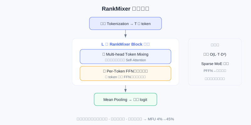
After input features are tokenized, they pass through multiple RankMixer Blocks (each = Token Mixing + Per-Token FFN), and mean pooling finally produces the logit. All core operations are matrix multiplications.
Each RankMixer Block's forward pass:
Overall complexity is . In the Sparse MoE version, the Per-Token FFN can be replaced with expert networks, expanding parameters while keeping inference cost. The design follows three principles: (1) all core operations are matrix multiplications, fully exploiting Tensor Cores; (2) the computation graph stays as simple as possible to reduce kernel launch overhead; (3) the expressiveness required by recommendation tasks is preserved.
7.4.1 The Token Mixing Mechanism
Self-Attention complexity is (from computing the full token-pair similarity matrix ). In recommendation, feature counts can reach hundreds or thousands, making the term a significant bottleneck. RankMixer's core insight: what recommendation tasks need is information mixing between tokens, not similarity-based dynamic weighting (attention). For example, learning high-order interactions like "young users in tier-1 cities prefer tech items" is essentially fusing information from multiple tokens into new representations — it does not necessarily require explicitly computing token-pair similarities.
Token Mixing's core idea: mix along the feature dimension rather than the token dimension. Given input , there are two steps:
Step 1, Multi-head decomposition — each token is decomposed into heads: , where is head of token .
Step 2, Token-wise mixing — within each head, concatenate that head's portion across all tokens: .
The key: change the data layout from "per token" to "per head". The original is vectors of length ; after SplitHead+Concat it becomes vectors of length , with different tokens' features densely packed within each head, creating the conditions for mixing. In practice , so each "head" holds a slice of every token's features. After mixing the token count is unchanged, enabling residual connections.
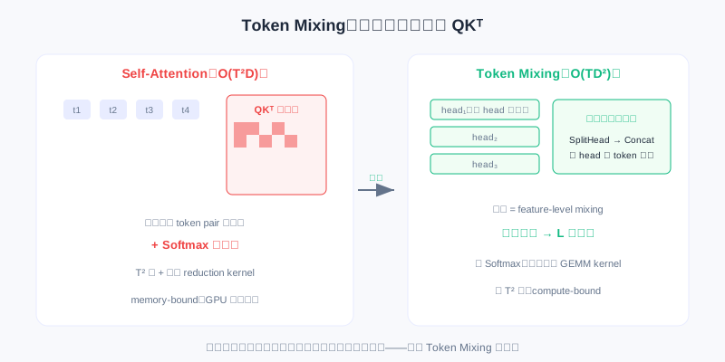
Left: Self-Attention computes the full similarity matrix (); right: Token Mixing rearranges by head and applies a linear transformation along the feature dimension (), with no softmax.
Complexity-wise, Token Mixing costs (mainly memory rearrangement). Compared with self-attention's , this avoids the term when is large (hundreds to thousands in recommendation) — a significant reduction. And Token Mixing has no softmax normalization (which requires an extra reduction kernel), further cutting kernel overhead.
The key question: without explicitly computing token-pair similarities, how are interactions still captured? The answer is stacking multiple layers. A single Token Mixing layer is "feature-level mixing" — the same feature dimension across tokens influences each other (because they are concatenated into one vector). With multiple stacked layers, layer 1's per-token output fuses first-order information from all tokens; layer 2's input is already a mixed result where each token contains other tokens' information, so layer 2's mixing achieves second-order interactions:
Each Token Mixing layer applies a linear transformation along the feature dimension (followed by FFNs), so stacking layers can model -th order polynomial interactions between tokens. In practice is usually 6–12 layers, enough to capture the needed high-order crossings.
From the hardware's perspective, Token Mixing's core is data rearrangement (SplitHead, Concat) that can be implemented with efficient kernels, designed as contiguous memory reads/writes (coalesced memory access) to fully use bandwidth. Compared with attention's softmax (a global normalization), Token Mixing is local and parallel. More importantly, SplitHead, Concat, and the FFN can be fused into a single kernel, reducing kernel launch overhead — the key to the MFU improvement.
Analysis: Token Mixing replaces "token-pair similarity + softmax" with "feature-dimension mixing + multi-layer stacking", dropping to overall, with all operations fusable into matrix-multiply kernels. What is sacrificed is attention's "dynamic similarity routing"; what is gained is GPU utilization — for recommendation, where features are numerous and interaction patterns fairly fixed, this trade is well worth it.
7.4.2 Per-Token FFN
The standard Transformer's FFN uses the same weights for all tokens: . This is reasonable for LLMs (all tokens share one semantic space). But recommendation features live in entirely different semantic spaces: user IDs imply implicit preferences, item categories are coarse-grained classes, click rates follow long-tail distributions, timestamps have periodicity. Forcing the same FFN on them loses parameter efficiency.
RankMixer's core design: each token gets its own FFN parameters. For the -th token:
Each token's is independent, so: (1) each token learns a transformation specific to its semantic space; (2) high-information tokens are automatically allocated more parameter capacity; (3) different semantic spaces no longer interfere.
Per-Token FFN is fundamentally different from MMoE. In MMoE, multiple experts share the same input, and gating dynamically weights a combination of expert outputs: (all experts see the same ). Per-Token FFN gives each token its own input and its own FFN: (each FFN sees a different ). Parameter isolation ensures learning in different feature spaces stays independent, preventing high-frequency features from dominating low-frequency ones.
For parameter efficiency, with tokens, Per-Token FFN has total parameters — times the shared FFN's (). But computational complexity is unchanged: , identical to the shared FFN (which must also compute once per token for tokens). The added parameters are "specialized" — each block serves only one token, giving higher learning efficiency.
Cross-feature-space interaction happens through the Token Mixing layers. Per-Token FFN focuses on deep modeling within each space; Token Mixing ensures information flows between tokens. This "mixing + per-token processing" combination preserves parameter isolation while achieving thorough cross-space interaction through multi-layer stacking.
7.4.3 Sparse MoE Scaling
With Token Mixing and Per-Token FFN in place, how do we scale to billions or even tens of billions of parameters? Directly adding depth/width scales compute linearly, and inference latency grows proportionally — industrially unacceptable. Sparse MoE (Sparse Mixture of Experts) provides the solution: not all parameters participate in every sample's computation; a subset of experts is dynamically selected per sample. The model can have a huge parameter count while per-sample compute stays fixed (activating only a few experts).
The ideal MoE pattern has each expert specialize in some sample pattern. But achieving effective expert specialization in recommendation faces three challenges: (1) the input is high-dimensional sparse features whose combinatorial space is exponential; representations are scattered across the high-dimensional space without clear cluster structure, making stable routing hard for the gating to learn; (2) data is extremely imbalanced — head users account for 50% of samples; if gating routes many head samples to one expert early on, that expert receives more gradients, gating keeps sending it more, and a few experts end up processing most samples (expert overload) while the rest go nearly unused (expert underutilization); (3) even if training is load-balanced, request distributions at inference may differ, making some experts bottlenecks and increasing latency variance.
RankMixer counters with two complementary training strategies. First, ReLU Routing — standard MoE uses Top- + Softmax routing, activating a fixed experts per token. RankMixer's ReLU Routing lets each token activate a variable number of experts:
ReLU outputs can be 0 (not activated) or positive (activated), so high-information tokens may activate more experts. To control sparsity, a regularization is added: , where and controls the average number of activated experts.
Second, Dense-Training / Sparse-Inference (DTSI-MoE) — Per-Token FFN already multiplies parameters by ; adding MoE on top expands expert count further, easily causing expert under-training. DTSI-MoE uses two routers: during training, a dense router activates all or most experts to ensure sufficient training; at inference, a sparse router activates only a few experts to cut compute. Both routers train simultaneously; only is constrained by :
During training, the forward pass uses while is computed alongside and given the sparsity regularization; at inference, only is used. This achieves sufficient training, efficient inference, and consistent strategy.
Load balancing is achieved through the soft constraint of . Expert 's total activation in a batch is , and the regularization can be rewritten as . When some expert's grows too large, the gradient suppresses its activation probability, achieving load balance. Compared with hard constraints (capacity limits), a soft constraint never force-assigns suboptimal experts when one is saturated, preserving routing flexibility.
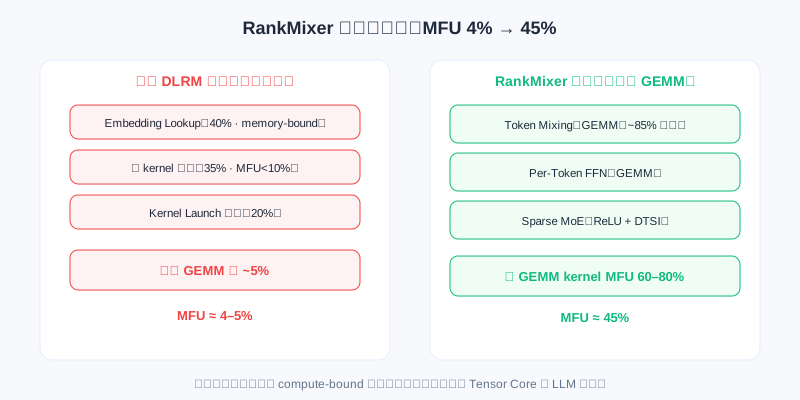
Left: the traditional DLRM's fragmented computation graph (memory-bound embedding lookups, small kernels, launch overhead), with effective GEMM at only 5%; right: RankMixer's core operations are all GEMMs — Token Mixing + PFFN take ~85% of compute, and MFU reaches 45%.
The key to RankMixer's high MFU: all core operations are compute-bound large matrix multiplications. Token Mixing and PFFN take about 85% of compute time, all GEMMs that efficiently use Tensor Cores (a single GEMM kernel reaches 60–80% MFU). By contrast, in the traditional DLRM, embedding lookups (40% of time, memory-bound), small kernels (35% of time, MFU<10%), and launch overhead (20% of time) dominate, with effective GEMM at only 5% — which is exactly why a DLRM's MFU is 4–5% while RankMixer reaches 45%.
💡 Key Insight: RankMixer moves the recommendation model from fragmented design to a unified architectural paradigm. Algorithmically, Token Mixing drops complexity from to , Per-Token FFN captures feature heterogeneity, and Sparse MoE achieves parameter-efficient scaling through ReLU Routing and DTSI-MoE. Systematically, unifying all core operations as matrix multiplications raises MFU from 4–5% to 45%, making the recommendation model a "first-class citizen" on GPU that can directly use Tensor Cores and the mature LLM toolchain, opening a path to sustained scaling. But RankMixer focuses on compute efficiency inside the model; the pipeline still has other fragmentation — sequence modeling separate from feature interaction, retrieval separate from ranking, multi-task fragmentation. The next section, OneTrans, breaks through these remaining walls.
⚠️ Common Mistakes in 7.4
| # | Mistake | Example | Why It's Wrong | Fix |
|---|---|---|---|---|
| 1 | Assuming low MFU just means few parameters | "Add GPUs and utilization is solved" | It is architectural fragmentation + memory-bound access, not a shortage of compute | Use hardware-aware unification into GEMMs |
| 2 | Assuming Token Mixing loses interactions | "Without token-pair similarity there are no crossings" | Multi-layer stacking achieves -th order polynomial interactions | Look at the stacking |
| 3 | Treating Per-Token FFN as MMoE | "One expert per token is just MoE" | MMoE shares the input and weights combinations; PFFN gives each token independent input/parameters | Distinguish parameter isolation from routed weighting |
| 4 | Using Top-k Softmax routing | "MoE should always activate a fixed k" | Sparse recommendation features make stable routing hard, and imbalance causes overload | Use ReLU Routing for dynamic activation |
| 5 | Ignoring the necessity of DTSI-MoE | "Just train sparse directly" | PFFN already multiplies parameters by T; pure sparse training under-trains experts | Two routers: dense training, sparse inference |
Chapter Summary
📌 Key Takeaways
| Concept | Key Points | Why It Matters |
|---|---|---|
| The MFU bottleneck | DLRM only 4–5%, LLM 40–60% | The hardware root cause of recommendation's scaling trouble |
| Token Mixing | Feature-dimension mixing replaces , complexity | Removes the term + fusable kernels |
| Per-Token FFN | Independent FFN parameters per token, unchanged complexity | Captures feature heterogeneity, parameter isolation |
| Sparse MoE | ReLU Routing + DTSI-MoE | Parameter-efficient scaling to the billion level |
| Unify as GEMM | All core operations are matrix multiplications | MFU up to 45%, a first-class GPU citizen |
❓ FAQ
Q1: Without computing similarities, can Token Mixing really replace Self-Attention?
A: Yes. High-order crossings in recommendation are essentially "fusing multiple tokens' information into new representations"; a single layer mixes along the feature dimension, and stacking layers achieves -th order polynomial interactions. The cost is losing dynamic similarity routing, but with many features and relatively fixed patterns in recommendation, the gained GPU utilization is the better deal.
Q2: Per-Token FFN multiplies parameters by T — why don't FLOPs change?
A: A shared FFN also computes once per token for T tokens (one FFN per token), so FLOPs were already ; Per-Token merely swaps the shared weights for T independent sets, still computing once per token — same FLOPs. What grows is "specialized" parameters with higher learning efficiency.
Q3: Why does recommendation MoE use ReLU Routing instead of Top-k?
A: Recommendation inputs are high-dimensional, sparse, and unevenly distributed; Top-k's fixed activation count easily overloads a few experts while the rest go underutilized. ReLU lets each token activate a variable number of experts based on information content, and with the regularization it achieves soft load balancing — better suited to recommendation data.
🔗 Connections to Later Chapters
- 7.3 (MTGR) — also handles heterogeneous features, but with GLN + Dynamic Masking; compare with RankMixer's Per-Token FFN (separate parameters) approach.
- 7.5 (OneTrans) — further breaks the fragmentation of "sequence modeling separate from feature interaction", extending RankMixer's hardware thinking to a unified architecture.
- 3.2 (Feature Crossing) — the high-order crossings of DCN/xDeepFM are re-implemented in RankMixer via multi-layer Token Mixing, and in a more GPU-friendly way.
Practice Problems
Work through all problems in order — they get progressively harder. Each has a complete solution you can reveal after trying it yourself.
Problem 7.4.1 — The Root Cause of Low MFU 🟢 Easy
A traditional DLRM's MFU is about 4–5%, an LLM's about 40–60%. Name the three architecture-level causes of the DLRM's low MFU.
💡 Solution (click to reveal)
Approach: Map to the three fundamental problems in the text.
- Core operations are memory-bound (embedding lookup, feature crossing — memory traffic >> compute);
- The computation graph is highly fragmented (many independent modules chained; kernel launch + global memory transfer overhead);
- Tensor Cores are underutilized (small vectors/irregular access, not GEMM).
Key points:
- It is not a lack of compute; the compute is not "worth it".
- RankMixer's unification into GEMM pulls MFU to 45%.
Problem 7.4.2 — Token Mixing Complexity 🟢 Easy
Self-Attention complexity is and Token Mixing about (rearrangement). With , by about how many times do the orders of magnitude differ?
💡 Solution (click to reveal)
Approach: Substitute and estimate (ignore constants).
- Self-Attention: .
- Token Mixing: .
- The ratio is x (i.e., times).
Key points:
- Token Mixing removes the term and scales linearly with token count.
- In recommendation, T is hundreds to thousands — the gain is significant.
Problem 7.4.3 — Per-Token FFN vs MMoE 🟡 Medium
Why are Per-Token FFN and MMoE "fundamentally different"? Summarize each one's parameter organization in a sentence.
💡 Solution (click to reveal)
Approach: Distinguish "parameter isolation" from "routed weighting".
- MMoE: multiple experts share the same input , and gating dynamically weights the output combination — all experts see the same input.
- Per-Token FFN: each token has its own input and its own FFN — parameter isolation, preventing high-frequency features from dominating low-frequency ones.
Key points:
- One is "same input, weighted expert selection"; the other is "different inputs, each with its own FFN".
- Both aim to handle heterogeneous features; the mechanisms differ.
Problem 7.4.4 — DTSI-MoE Design 🔴 Hard
Explain why DTSI-MoE needs two routers ( and ), and what would happen if you trained with only .
💡 Solution (click to reveal)
Approach: Start from the tension between "sufficient training vs efficient inference".
Per-Token FFN already multiplies parameters by T, and MoE expands the expert count further; if training also activates sparsely, many experts never receive enough gradients → expert under-training. DTSI-MoE uses during training to activate most experts (sufficient training), while only is constrained by the sparsity regularization and used at inference. Training with only would under-train the experts, and the deployed model would perform poorly.
Key points:
- Dense training preserves quality; sparse inference preserves efficiency.
- The two routers train simultaneously with a consistent strategy.
🏆 Challenge: Hardware-Aware Restructuring
You must restructure a fragmented DLRM (embedding lookup + hand-crafted crossing + DIN + MLP) into a GPU-friendly architecture. Within 150 words, state which three RankMixer components you would substitute for the existing modules, and the expected MFU change plus its precondition.
💡 Hint
Replace Self-Attention/hand-crafted crossing with Token Mixing (removes , fusable kernels), replace the shared FFN with Per-Token FFN (captures feature heterogeneity), and scale parameters with Sparse MoE. The precondition is first tokenizing all features and unifying the computation graph as matrix multiplications; expect MFU to rise from ~5% to ~45%. This corresponds exactly to RankMixer's hardware-aware restructuring approach.
OneTrans: Unifying Sequence Modeling and Feature Interaction
📝 Before You Continue: You have read 7.4 RankMixer (compute efficiency within the model). This chapter goes further — tearing down the architectural wall between the "sequence modeling module" and the "feature interaction module", doing end-to-end joint optimization with a single Transformer backbone and reusing LLM system optimizations.
RankMixer solved the GPU utilization problem through hardware-aware design, but the overall recommendation system architecture remains fragmented. Mainstream industrial recommenders widely adopt the encode-then-interaction paradigm: a sequence modeling module (DIN, LONGER) encodes the behavior sequence into a fixed-length vector, which is then concatenated with non-sequential features and fed into a feature interaction module (such as RankMixer) to learn high-order crossings.
This separated design has two fundamental problems: (1) restricted information flow — the sequence must be compressed into a fixed-dimension vector, static features cannot play a role during sequence encoding, and can only be fused in later as a "remedy"; (2) fragmented execution — the two modules execute independently and cannot benefit from LLM system optimizations (KV Caching, FlashAttention), and each requires separate tuning, making a unified Scaling Law hard to form.
OneTrans proposes a fundamental architectural renovation: accomplish both sequence modeling and feature interaction with a single Transformer backbone. A unified tokenizer converts sequential features (S-tokens) and non-sequential features (NS-tokens) into a unified token sequence, jointly modeled in stacked Transformer layers — breaking the information wall between sequences and features, and laying the foundation for applying LLM system optimizations.
7.5.0 Unified Tokenization
Recommendation inputs contain two very different kinds of features: sequential features (the user's multiple behavior sequences, such as clicks, add-to-cart, and orders) and non-sequential features (static attributes and context, such as age, category, query terms, hour). Traditional methods compress into a fixed vector and concatenate it with ; OneTrans's core innovation is converting both kinds of features into a unified token sequence, processed in the same Transformer.
For sequential features ( behavior types), each sequence contains event embeddings (event = item ID + item-side information). Since the raw dimensions of different behavior sequences may differ, a behavior-specific MLP first aligns them to a unified dimension :
After alignment, the multiple sequences must be merged into a single token sequence. OneTrans supports two fusion strategies: (1) Timestamp-aware — if behaviors carry timestamps, interleave all behaviors by time and add behavior-type identifiers; (2) Timestamp-agnostic — if there are no timestamps, sort by behavioral intent strength (order > add-to-cart > click), inserting learnable [SEP] tokens between different sequences. Experiments show timestamp-aware works better when timestamps exist (temporal ordering encodes interest evolution). Finally:
For non-sequential features (numerical and categorical features, embedded after bucketization or one-hot), OneTrans concatenates all features, projects them through a single MLP, and then splits into tokens (called the Auto-Split Tokenizer):
This avoids the subjectivity of manual feature grouping, letting the model learn how to organize non-sequential features on its own. The final initial input is the concatenation of S-tokens and NS-tokens:
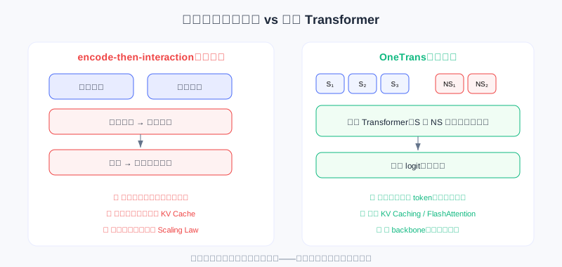
Left: the traditional separated approach (the sequence is encoded into a fixed-length vector then concatenated with static features, restricting information flow); right: OneTrans's unified token sequence, with S-tokens and NS-tokens jointly modeled in the same Transformer.
This differs essentially from traditional methods: they compress the sequence into a single vector, while OneTrans keeps the full sequence tokens. In subsequent Transformer layers, each behavior event participates in attention as an independent token, non-sequential features also exist in token form, and the two kinds of features can interact within the same attention matrix.
7.5.1 The Core Mechanism of Mixed Parameterization
Directly processing the unified token sequence with a standard Transformer runs into a recommendation-specific difficulty: token heterogeneity. In an LLM, all tokens are words/sub-words in one semantic space, so sharing Q/K/V and the FFN is reasonable. But in OneTrans, S-tokens come from behavior sequences (strongly homogeneous — all user-item interaction events), while NS-tokens come from entirely different spaces (age is demographic, price is numerical, query is text). Forcing all tokens to share parameters creates conflicts — for example, parameters that capture "similarity of adjacent items in the sequence" may be completely unsuited to the "user age → item category" interaction.
OneTrans's core innovation is Mixed Parameterization: S-tokens share one set of parameters, while each NS-token gets its own token-specific parameters. This rests on two observations: (1) all events in the behavior sequence live in one semantic space (the item space), so sharing parameters to learn sequential patterns is efficient; (2) non-sequential features come from heterogeneous spaces and need independent parameters to capture their individual characteristics.
Mixed Causal Attention
The Q/K/V of Multi-Head Attention in an OneTrans Block use mixed parameterization. The query/key/value of the -th token :
The weight matrices follow conditional parameterization:
All S-tokens use the same ; the -th NS-token has its own and so on.
OneTrans adopts a Causal Attention Mask, with NS-tokens placed after S-tokens, producing three key information-flow patterns:
- S-side causal dependency — each S-token can only attend to preceding S-tokens. Timestamp-aware naturally models temporal causality; under timestamp-agnostic (sorted by intent), the causal mask lets high-intent behaviors (orders) pass information to low-intent ones (clicks), achieving "strong signals filtering weak signals".
- NS-side global attention — each NS-token can attend to all S-tokens (the full behavior history) plus preceding NS-tokens. This lets non-sequential features fully exploit sequential evidence — e.g., the "item category" token can attend to all historical click categories and automatically learn "the user's historical preference for this category".
- Support for the Pyramid — the causal mask's directionality makes information naturally converge toward the tail of the sequence, providing the theoretical basis for the Pyramid Stack.
Mixed FFN
The FFN likewise uses mixed parameterization:
follow the same conditional parameterization as attention: S-tokens share , while each NS-token is independent.
A comparison with RankMixer's Per-Token FFN is needed: RankMixer gives every token its own FFN (including sequence tokens), with parameters ; OneTrans's Mixed FFN assigns independent parameters only to the NS-tokens while S-tokens share, with parameters . In recommendation , so OneTrans significantly cuts parameter overhead while preserving expressiveness. Parameter sharing is not a compromise — it is the design — the homogeneity of behavior sequences makes shared parameters more efficient at learning sequential patterns and avoids redundancy.
OneTrans uses Pre-norm + RMSNorm. S-tokens and NS-tokens differ significantly in numerical range/statistics; Post-norm easily causes attention score scale imbalance and unstable training; Pre-norm normalizes before each sublayer, ensuring token representations entering attention/FFN have similar scales, and RMSNorm further provides more stable gradient propagation through root-mean-square normalization.
S-tokens share Q/K/V/FFN parameters with causal dependency; NS-tokens have independent parameters and can globally attend to all S-tokens. The two feature types interact in the same attention matrix.
7.5.2 Pyramid Stack: Progressive Distillation
OneTrans's Causal Attention has an important property: information naturally converges toward the back of the sequence. Position at layer fuses information from ; position at layer then fuses the updated . As depth increases, later tokens gradually become "convergence points" holding all preceding tokens' information. In particular, NS-tokens sit at the sequence's end, so deep layers accumulate the whole sequence plus preceding NS-tokens' information.
The Pyramid Stack exploits this: layer by layer, reduce the number of query tokens participating in attention, keeping only the tail of the sequence. Suppose layer 's input has length ; define the tail index set (). The attention computation:
- Keys and Values: still computed from all tokens, preserving full context
- Queries: computed only from the tokens in
The attention output keeps only the positions corresponding to , shrinking sequence length from to . Across layers, use decreasing (e.g., 1190 → 595 → 297 → … → 12), forming a pyramid-style hierarchy.
Each layer's queries take only the tail tokens (including NS-tokens); Keys/Values use all tokens; sequence length halves layer by layer, progressively distilling information toward the tail.
Two core benefits:
- Progressive Distillation — long behavior sequences (hundreds or thousands of events) shrink layer by layer, with information gradually "distilled" into a small number of tail tokens. Shallow layers learn local patterns (adjacent item similarity); deep layers learn global patterns on the compressed tokens (long-term interest drift). Finally all sequence information converges into the NS-tokens, providing a compact yet information-rich representation for downstream use.
- Compute Efficiency — standard Transformer attention complexity is and FFN . The Pyramid drops these to (attention) and (FFN). When (e.g., 1190 shrinking to 12 layer by layer), compute and activation memory fall significantly.
The key difference from a standard Transformer: the standard one must maintain the full sequence length at every layer (LLMs need per-position predictions); recommendation only needs the final ranking score, so intermediate sequence tokens can be discarded layer by layer, as long as the tail tokens have fully fused the history. The causal attention's directionality guarantees this.
7.5.3 Cross-Request KV Caching
A key advantage of the unified architecture is that LLM system optimizations apply seamlessly — most importantly KV Caching. A single request usually returns hundreds of candidates, each corresponding to one sample; these samples share identical user-side features (same user, same behavior sequence), differing only on the item side. Under traditional encode-then-interaction, the sequence encoding module can be reused, but the feature interaction module must be recomputed for every candidate — the shared structure goes underused.
OneTrans's unified Transformer naturally supports two-stage computation:
Stage I (S-side, once per request) — process all S-tokens, computing each layer's K/V and attention output and caching them. This stage executes once per request, independent of candidate count.
Stage II (NS-side, per candidate) — for each candidate, compute its NS-tokens; at each layer: use the cached S-side K/V, compute the NS-tokens' queries, run Cross-Attention (NS attends to the cached S-side K), run Self-Attention among NS-tokens, and process the NS-tokens through token-specific FFNs.
The key: the S-tokens' KV is shared across all candidates; only the NS-tokens' QKV needs recomputing per candidate. With candidates per request, the traditional approach needs sequence computation; KV Caching drops it to . Since , complexity is approximately with respect to candidate count .
Going further, OneTrans implements Cross-Request KV Caching. User behavior sequences are append-only; each new request appends only a few events at the end compared to the last. The KV cache can be reused across requests:
- First request — compute and cache the full sequence's KV
- Subsequent requests — compute only the KV of the newly added events and concatenate with the old cache
Per-request sequence computation drops from to ( is usually single-digit). In high-frequency scenarios (feed refreshes) where the user sequence changes little in a short window, Cross-Request KV Caching pays off especially well.
Stage I computes and caches the S-side KV once per request; Stage II computes only the NS-side per candidate; across requests, only the KV of the newly appended events is computed, reusing the old cache.
Note that KV Caching's effectiveness depends on the unified Transformer computation graph. If sequence modeling and feature interaction are two separate modules, their intermediate representations cannot be reused across candidates (inputs/parameters differ completely). OneTrans, through unified tokenization and Mixed Parameterization, places both feature types in the same attention matrix so the S-tokens' KV can be shared by all candidates' NS-tokens — something encode-then-interaction cannot achieve.
Beyond KV Caching, OneTrans inherits other LLM optimizations: FlashAttention-2 (kernel fusion + memory tiling to cut attention I/O and activation memory), Mixed-Precision Training (BF16/FP16) combined with Activation Recomputation (preserving numerical stability while compressing memory). These matter greatly for training and deploying OneTrans with hundreds of millions of parameters.
7.5.4 The Essence of Unified Modeling
OneTrans's core contribution is a fundamental shift in recommendation architecture: from composing modules to unified modeling. Traditional encode-then-interaction splits sequence encoding and feature interaction into separate modules, artificially severing different interaction types (within-sequence, cross-sequence, multi-source features, sequence-feature). OneTrans's unified Transformer lets these interactions happen simultaneously at every layer, with multi-layer stacking forming complex combinatorial patterns.
Another key advantage of the unified architecture is overall scalability. A separated architecture requires separately tuning the sequence and interaction modules, making a unified Scaling Law hard to form. OneTrans unifies the whole model into a single Transformer backbone with a simple, clear scaling strategy: add layers (depth), add hidden dimensions (width), add sequence length — recommendation models can gain predictable performance improvements just like LLMs.
From RankMixer to OneTrans, recommendation architecture evolution shows two clear directions: hardware-aware computation design solves GPU utilization, and a unified modeling framework breaks the walls of module fragmentation. Together they lay the foundation for recommendation systems to move toward large-scale, scalable intelligence.
💡 Key Insight: This chapter closes Part 7 — from HSTU validating the Scaling Law, to GenRank probing the essence, MTGR reconciling features, RankMixer optimizing hardware, and OneTrans unifying the architecture. From the five angles of architecture, training, features, hardware, and unification, the five works jointly prove: recommendation systems are no longer the "exception" to deep learning scaling.
⚠️ Common Mistakes in 7.5
| # | Mistake | Example | Why It's Wrong | Fix |
|---|---|---|---|---|
| 1 | Assuming OneTrans is just RankMixer reskinned | "They're all Transformers, no difference" | OneTrans tears down the sequence/feature module wall and unifies tokens | Distinguish "efficiency within the model" vs "architectural unification" |
| 2 | Letting all tokens share parameters | "A unified sequence just uses a standard Transformer" | S/NS tokens are heterogeneous; shared parameters conflict | Use Mixed Parameterization (S shared / NS independent) |
| 3 | Compressing the sequence into a fixed-length vector | "Pool S-tokens first, then append NS" | Loses per-event interaction, back to encode-then-interaction | Keep the full sequence tokens, interacting in the same attention |
| 4 | Ignoring the Pyramid's causal precondition | "Just truncate queries arbitrarily" | The causal mask is needed to guarantee tail convergence of history | Keep only the tail queries, KV uses all |
| 5 | Assuming KV Cache works in a separated architecture too | "DIN+RankMixer can also reuse across candidates" | The two modules' inputs/parameters differ; intermediate representations can't be reused across candidates | A unified computation graph is the prerequisite for Cross-Request KV Cache |
Chapter Summary
📌 Key Takeaways
| Concept | Key Points | Why It Matters |
|---|---|---|
| Unified Tokenization | S-tokens (sequential) + NS-tokens (non-sequential) in one sequence | Breaks the sequence/feature information wall |
| Mixed Parameterization | S shared parameters / NS independent parameters | Resolves token heterogeneity conflicts |
| Pyramid Stack | Queries shrink to the tail layer by layer, KV uses all | Progressive distillation + compute efficiency |
| Cross-Request KV Cache | S-side KV reused across candidates/requests | Complexity near (relative to candidates) |
| Essence of unified modeling | Single Transformer backbone, jointly optimized | Overall scalability, forming a unified Scaling Law |
❓ FAQ
Q1: What is the biggest difference between OneTrans and RankMixer?
A: RankMixer focuses on compute efficiency within the model (Token Mixing replacing attention, 45% MFU) but still treats sequence and features as separable inputs; OneTrans goes further, unifying sequence events and non-sequential features into a token sequence, jointly modeled inside one Transformer, and reuses LLM system optimizations such as KV Caching.
Q2: Why do S-tokens share parameters while NS-tokens are independent?
A: All events in the behavior sequence live in one "item space" with high homogeneity — shared parameters learn sequential patterns more efficiently and avoid redundancy; non-sequential features come from heterogeneous spaces (demographics/numerical/text) and need independent parameters to capture their characteristics. This is "parameter sharing as design, not compromise".
Q3: Why can the Pyramid Stack discard intermediate tokens?
A: Recommendation only needs the final ranking score — unlike LLMs, it does not need per-position predictions. Causal attention makes information converge toward the tail; keeping the tail queries (including NS-tokens) with KV using all tokens cuts compute dramatically without losing historical information.
🔗 Connections to Later Chapters
- 7.1 (HSTU) — M-FALCON first proposed using KV caching to decouple history from candidates; OneTrans's Cross-Request KV Caching extends that idea on a unified architecture.
- 7.4 (RankMixer) — its hardware efficiency is the base that makes OneTrans's unified architecture scalable; together they point toward "recommendation models as first-class GPU citizens".
- Part 6 Generative Fundamentals and Part 8 End-to-End Generation push the unified modeling idea across the full "retrieval–ranking–re-ranking" pipeline — continue reading along that line.
Practice Problems
Work through all problems in order — they get progressively harder. Each has a complete solution you can reveal after trying it yourself.
Problem 7.5.1 — Paradigm Identification 🟢 Easy
Determine whether each description belongs to "encode-then-interaction (separated)" or "OneTrans (unified)":
- (a) DIN encodes the behavior sequence into a fixed-length vector, then concatenates it with static features into the crossing module
- (b) Behavior events and non-sequential features are all tokens, jointly attending at every layer of the same Transformer
💡 Solution (click to reveal)
Approach: Grasp "does it keep full sequence tokens, and do both types interact within the same layer".
- (a) Separated (encode-then-interaction): the sequence is compressed into a fixed-length vector and concatenated later.
- (b) OneTrans unified: both feature types are tokens interacting in the same attention matrix.
Key points:
- The core of unified modeling is "no sequence compression, same-layer interaction".
- The restricted information flow of the separated approach is exactly the pain point OneTrans solves.
Problem 7.5.2 — Mixed Parameterization 🟢 Easy
How does parameter organization differ between S-tokens and NS-tokens in OneTrans? Why this design instead of sharing everything?
💡 Solution (click to reveal)
Approach: Map directly to Mixed Parameterization.
- S-tokens (behavior sequence) share one set of Q/K/V/FFN parameters (same item space, homogeneous).
- NS-tokens (non-sequential features) each have independent parameters (heterogeneous spaces).
- Sharing everything would make heterogeneous tokens' parameters conflict (e.g., "adjacent item similarity" parameters don't fit "age → category").
Key points:
- Parameter sharing is design (sequence homogeneity), not compromise.
- Compared with RankMixer's per-token independent FFNs, OneTrans saves parameters because .
Problem 7.5.3 — Pyramid Complexity 🟡 Medium
For a sequence of length , a standard Transformer's attention complexity is . The Pyramid Stack takes the tail as queries per layer (let ), with KV using all . With 4 stacked layers ( halving from 1190 down to about 12), what fraction of the standard Transformer's total attention compute (same 4 layers, full length throughout) does the Pyramid roughly cost?
💡 Solution (click to reveal)
Approach: Each Pyramid layer's attention is ; each standard layer is .
Estimate (KV fixed at full length ): the Pyramid layers' query lengths are about , so the 4-layer total is . Compared with the standard 4 layers' , this is roughly 1/4.
In practice even lower: each layer's KV sequence also shrinks with depth, so each layer costs , which is smaller than the formula above; the true ratio is slightly below .
Key points:
- The point is not the exact multiple but the square-to-linear order drop from "shrinking queries layer by layer".
- At inference you can give the order-of-magnitude conclusion: significantly below the standard Transformer.
Problem 7.5.4 — KV Cache Payoff 🔴 Hard
A request has candidates, sequence tokens, . The traditional per-candidate sequence computation is about ; OneTrans with Cross-Candidate KV Caching is about . By about how many times do the orders of magnitude differ?
💡 Solution (click to reveal)
Approach: Substitute and estimate (ignoring the constant ).
- Traditional: .
- OneTrans: .
- The ratio is x.
Key points:
- S-side KV is computed once across candidates; complexity is near relative to .
- Because , the payoff grows as candidate count grows.
🏆 Challenge: A Unified Architecture Blueprint
Within 150 words, drawing on the five works in Part 7, describe the four characteristics your ideal "scalable recommendation ranking engine" should have (one each from paradigm, features, hardware, and architectural unification).
💡 Hint
The four characteristics: (1) paradigm — user-level autoregressive sequence modeling (the essence of HSTU/GenRank); (2) features — retain cross-feature compatibility (MTGR's hybrid paradigm); (3) hardware — unify into matrix multiplications, 45% MFU (RankMixer hardware-aware); (4) architectural unification — a single Transformer backbone jointly modeling sequence and feature interaction + KV Caching (OneTrans). These correspond exactly to the combined direction of Part 7's five works.
For over a decade, recommendation, search, and advertising have almost all been built on the Multi-stage Cascading Architecture (MCA): retrieval, pre-ranking, ranking, re-ranking... data is filtered layer by layer like a funnel. This design historically balanced efficiency and complexity, but as data scales exploded and user-experience expectations rose, its structural flaws became increasingly apparent — conflicting objectives, information loss, and fragmented computation.
This part stops treating each sub-task in isolation. Instead, along the generative paradigm thread, we look at how industry uses a unified neural network to generate final results directly from user input, completely overturning the "cascading funnel." We focus on real deployments in three core business scenarios: Kuaishou's OneRec (end-to-end generative recommendation), e-commerce search's OneSug + OneSearch (end-to-end generative search), and online advertising's EGA + GPR (end-to-end generative advertising).
💡 Key Insight: The end-to-end practices across the three scenarios share one common thread — semantic IDs are the bridge connecting generative models to business data; the Encoder-Decoder is the workhorse architecture for fusing context; and reinforcement learning is the key tool for aligning the generation process with online business objectives.
What This Part Covers
| Section | Topic | The Big Idea |
|---|---|---|
| 8.1 | End-to-End Generative Recommendation | OneRec-V1/V2 use semantic IDs + Encoder-Decoder + reinforcement learning to redefine recommendation as a generation task: "user context → semantic ID sequence" |
| 8.2 | End-to-End Generative Search | OneSug handles query completion and OneSearch handles product retrieval, covering the full e-commerce search pipeline with a unified generative architecture |
| 8.3 | End-to-End Generative Advertising | EGA embeds the auction mechanism into generation and GPR uses pre-training to unify ultra-long heterogeneous sequences across scenarios, deeply integrating mechanism constraints with the generative model |
What You'll Be Able to Do After This Part
- 🟢 Explain the three structural flaws of the traditional MCA and how they gave rise to the end-to-end generative paradigm
- 🟢 Describe how semantic IDs compress hundreds of millions of items into a finite vocabulary, making generative recommendation mathematically feasible
- 🟡 Contrast the fundamental difference in compute allocation between OneRec-V1's Encoder-Decoder and V2's Lazy Decoder-Only
- 🟡 Distinguish the essential difference between the search scenario's "relevance first, personalization second" and the recommendation scenario's optimization objective
- 🔴 Explain how EGA embeds incentive compatibility (IC) and individual rationality (IR) constraints into the generation process
- 🔴 Outline how GPR's heterogeneous hierarchical decoder and value-guided Beam Search solve the cross-scenario and ultra-long-sequence challenges
- 🏆 Complete the tiered practice problems in each section, working through semantic ID encoding, reward modeling, and constrained decoding by hand
Core Concepts
| Concept | Section | Relevance |
|---|---|---|
| Multi-stage Cascading Architecture (MCA) | 8.1 | The traditional industrial skeleton overturned by the end-to-end paradigm |
| Semantic ID | 8.1 | The core bridge connecting generative models to discrete items/products/ads |
| Encoder-Decoder generative architecture | 8.1 / 8.2 / 8.3 | The workhorse structure for fusing context and autoregressively generating sequences |
| Lazy Decoder-Only | 8.1 | Concentrates compute on target tokens, cutting decoding cost by 94% |
| RL alignment (ECPO/GBPO/DPO) | 8.1 / 8.2 / 8.3 | Aligns the generation process with online multi-objective business signals |
| Incentive compatibility (IC) and individual rationality (IR) | 8.3 | Economic constraints from mechanism design in the advertising scenario |
| Value-guided Trie Beam Search | 8.3 | Embeds constraints into decoding and improves inference efficiency |
Prerequisites
- You have finished 1.1 (the two paradigms and the motivation for end-to-end generation) and 2.x (two-tower models and a first look at semantic IDs)
- Familiarity with the basic Transformer structure (self-attention, cross-attention, encoder/decoder)
- A preliminary understanding of reinforcement learning basics (policy, reward, advantage) — this part develops them gradually through case studies
This part is the industrial-deployment chapter of the generative thread and leans Advanced — there are many formulas, but remember: better to lean on the figures than to wrestle with the formulas. The point is to understand the "why" behind each architectural choice.
Tips for This Part
- Follow the hidden thread of "semantic IDs." All three sections — recommendation, search, advertising — repeatedly solve the same problem: how to turn discrete business objects into token sequences a generative model can "speak out." Understand semantic IDs first and the rest follows naturally.
- Read the three sections comparatively. Each follows "MCA pain points → generative solution → alignment with online objectives," but the business constraints differ: recommendation pursues interests, search protects relevance first, and advertising must additionally satisfy economic mechanisms.
- Pay attention to the engineering trade-offs between compute and constraints. OneRec-V2's Lazy architecture and GPR's Trie-constrained decoding are both classic examples of trading architecture for efficiency and compliance.
Let's dive in! 🚀
End-to-End Generative Recommendation
📝 Before You Continue: This chapter assumes you understand the two paradigms and the motivation for end-to-end generation from 1.1, and are familiar with the introductory concept of semantic IDs from 2.3. This chapter pushes them to industrial-scale deployment.
The traditional multi-stage cascading architecture (MCA) exposes its sharpest contradictions in recommendation: massive compute is consumed by communication and storage rather than model computation, leaving GPU utilization far below that of large language models; each stage has scattered objectives, and divergent model structures cause inconsistent modeling; the cascade further blocks the application of advanced techniques such as Scaling Laws and RL alignment.
Kuaishou's OneRec framework redefines recommendation as an end-to-end generative task: the model directly "generates" a recommendation sequence from user context instead of "selecting" from a candidate pool. This section first examines the deep bottlenecks of the cascading architecture, then walks through the OneRec-V1 system and how V2 breaks through those bottlenecks.
After reading this chapter, you will be able to:
- Explain how semantic IDs solve the "Softmax explosion from directly generating atomic IDs" problem
- Describe OneRec-V1's four-pathway encoder and reward system design, along with the two bottlenecks it faces
- Explain why the Lazy Decoder-Only cuts decoding computation by 94%
- Recount the validation of Scaling Laws on OneRec-V2 and GBPO's improvements over ECPO
- Complete 5 tiered practice problems consolidating semantic IDs, architecture, and alignment algorithms
8.1.0 Why End-to-End Generative Recommendation
Recommender systems have long run on the "retrieval — pre-ranking — ranking — re-ranking" funnel. But as described in 1.1, the cascading architecture has three persistent pain points, especially acute in recommendation:
- Computation fragmentation — each stage is deployed and communicates independently, so massive resources go to data transfer rather than useful computation; GPU utilization is far below LLM training.
- Conflicting optimization objectives — retrieval optimizes relevance, ranking optimizes CTR, re-ranking optimizes diversity; each fights its own battle, yielding global sub-optimality with errors accumulating layer by layer.
- Disconnect from the AI frontier — stage fragmentation makes it hard to directly import techniques validated at scale in the LLM world, such as Scaling Laws and RLHF.
💡 Key Insight: The essence of the end-to-end generative architecture is not "swap in a bigger model," but re-converging scattered sub-objectives into one unified sequence-generation loss, thereby making global optimality possible.
🧠 Mental Model: From "Talent-Show Judge" to "Personal Tailor"
Think of cascaded recommendation as a talent show: thousands of contestants pass a first screen (retrieval), then judges score them one by one (ranking), and finally the director arranges the running order (re-ranking). Every step "shrinks the candidate pool." End-to-end generation is like a tailor who knows your taste — instead of listening to you list candidates, he directly cuts a garment (generates a sequence) from your measurements (context). Fewer intermediate steps, less distortion.
8.1.1 Semantic IDs: Letting the Model "Speak" an Item
The first hard nut generative recommendation must crack is: how does a model "speak" an item? Traditional systems identify items with atomic IDs (e.g., video ID vid_12345678), but Kuaishou has billions of items, and directly generating atomic IDs would blow up the Softmax layer's computation.
OneRec-V1 adopts semantic IDs: mapping items into a finite, controllable vocabulary space. Each video is encoded as semantic tokens with vocabulary size . The total encoding space is — far larger than the actual item count, which both guarantees coverage and uses the larger vocabulary to introduce more parameters for better performance.
Generating semantic IDs happens in two stages:
Stage one: collaboration-aware multimodal representation learning. A video's title, tags, ASR, OCR, cover, and sampled frames are compressed by a vision-language model (e.g., miniCPM-V-8B) into 1280 tokens, then compressed by a QFormer into 4 learnable query vectors. But relying on content features alone cannot capture collaborative signals, so item-pair contrastive learning is introduced to pull together item pairs with high collaborative similarity:
A title-generation auxiliary task is used concurrently to prevent representation collapse and preserve content understanding.
Stage two: RQ-Kmeans hierarchical quantization. After obtaining collaboration-aware representations, residual-quantized K-means (RQ-Kmeans) discretizes the continuous representations into semantic IDs. Unlike end-to-end-trained RQ-VAE, RQ-Kmeans directly runs K-means on residuals to build codebooks:
After 3 quantization layers, each video gets a coarse-to-fine semantic identifier sequence , which becomes the generative model's output target.
Analysis: Semantic IDs are the bridge between the "generative model" and "discrete items." They compress a mega-vocabulary down to a controllable size, while letting semantically similar items share prefix tokens — which benefits both generation and the subsequent coarse-to-fine hierarchical decoding. The cost is that quantization is lossy, so codebooks need careful design.
8.1.2 OneRec-V1: Encoder-Decoder and Preference Alignment
With semantic IDs in hand, OneRec-V1 uses the classic Encoder-Decoder architecture for end-to-end generation: the encoder processes the user's multi-scale features, and the decoder generates the target item's semantic ID sequence autoregressively given the context.
Encoder: Four Pathways for Understanding the User
The encoder embodies a deep understanding of user interests at multiple time scales, with four pathways:
- User static-feature pathway — basic profile such as ID, age, gender, passed through two dense layers to get .
- Short-term behavior pathway — the most recent interactions, including item/author IDs, tags, timestamps, watch duration, and interaction labels, yielding .
- Positive-feedback behavior pathway — the most recent high-engagement interactions, yielding .
- Ultra-long-term history pathway — a major OneRec-V1 innovation. A user can have up to 100,000 history records; processing them directly would explode compute. First, hierarchical K-means compresses them (with clusters selecting representative items), then a QFormer applies cross-attention over the compressed sequence of length 2000 with 128 learnable queries, yielding .
The four pathways' outputs are concatenated and passed through Transformer encoder layers:
The final output provides comprehensive context.
Decoder: Autoregressive Semantic ID Generation
The decoder's input is [BOS] plus the target item's semantic ID sequence; each layer contains causal self-attention (capturing dependencies among generated tokens), cross-attention (attending to the encoder's context), and MoE feed-forward (top-k routing to add capacity while keeping efficiency). Training uses the cross-entropy of next-token prediction:
Reward System: Breaking the "Imitation Ceiling"
Pre-training only fits the historical exposure distribution, and exposure data comes from the traditional system — the model is essentially "imitating" the past, with its performance ceiling shackled by the old system. OneRec-V1 introduces reward-system-based RL post-training with three reward components:
① User preference alignment (P-Score). A neural network learns personalized preference scores. Built on the SIM architecture, it erects an independent tower for each objective (CTR, LTR, VTR, etc.); each tower trains with binary cross-entropy on its corresponding label as an auxiliary task, then feeds a final MLP that outputs the P-Score:
② Generation format regularization (format reward). The semantic ID encoding space is far larger than the item count, so inference may generate illegal sequences that map to no real item. Introducing RL sharply worsens this — due to the Squeezing Effect: the model squeezes probability mass onto the current best output, pressing some legal tokens' probabilities down to levels close to illegal tokens'. OneRec-V1 sets the advantage to 1 for legal samples and directly discards illegal samples to avoid squeezing.
③ Industrial-scenario alignment (SIR). The end-to-end property means you "just need to fold optimization objectives into the reward system." For example, when viral content exceeds a fraction threshold , down-weight the P-Score:
Experiments show SIR reduced viral-content exposure by 9.59% with core metrics stable.
ECPO: The Preference Alignment Algorithm
OneRec-V1 aligns preferences with ECPO (Early Clipped GRPO). For user , the old policy generates items, each scored by P-Score to get reward :
The advantage is , and the old policy is early-clipped:
ECPO's key improvement is pre-clipping the policy ratio for negative-advantage samples, avoiding the exploding gradients that arise in GRPO when the ratio for negative advantages grows arbitrarily large.
Analysis: V1 validated the feasibility of end-to-end generative recommendation on Kuaishou's production system. But scaling up the model exposed two bottlenecks: first, the Encoder-Decoder's imbalanced compute allocation — the overwhelming majority of compute goes to context encoding, while decoding the target tokens, which actually produce gradients, accounts for a tiny fraction; second, reward-model-based RL suffers from low sampling efficiency and reward-hacking risk. These gave birth to V2.
8.1.3 OneRec-V2: Lazy Decoder-Only and Scaling Laws
OneRec-V2 breaks through along two dimensions: architecturally, it proposes the Lazy Decoder-Only to solve compute efficiency; algorithmically, it introduces RL based on real user feedback to break the reward-model limitation.
Lazy Decoder-Only Architecture
The design philosophy: concentrate compute on the target-item tokens that actually contribute gradients to the loss. It has two core components:
Context Processor. All user features are concatenated into a unified context sequence, with each token mapped to dimension:
where is the key-value separation coefficient ( shared, separated) and is the number of key-value layers. The Context Processor slices along the feature dimension into groups, each generating key-value pairs via RMSNorm. The clever part: these key-value pairs are invariant for the same context throughout, so they can be shared across decoder layers — no recomputation per layer. Even with extreme sharing (), performance doesn't visibly degrade.
Lazy Decoder Block. Unlike a traditional Decoder-Only that concatenates all inputs into one long sequence for self-attention, it does not treat the context as part of the sequence, but rather as static conditional information accessed only via cross-attention. "Lazy" means: the loss is computed only at target-token positions, not as an NTP loss at every position of the whole sequence.
During training, the target item's first two semantic IDs plus [BOS] form an input sequence of just 3 tokens:
Each layer has three steps: Lazy Cross-Attention (no key-value projection; uses GQA grouped queries to reduce memory), Causal Self-Attention (autoregression among semantic IDs), and FFN (deep layers may swap in MoE).
Quantifying the Efficiency Gain
Through this design, the Lazy Decoder-Only achieves nearly 100% of computation concentrated on target tokens:
| Architecture | Parameters | Computation (GFLOPs) | Converged Loss |
|---|---|---|---|
| Encoder-Decoder (1:1) | 1B | 296.36 | 3.28 |
| Lazy Decoder-Only | 1B | 18.89 | 3.27 |
In other words, at comparable performance, computation drops by 94% and training resources are saved by 90%.
Validating the Scaling Law
The Lazy Decoder-Only exhibits excellent scalability. OneRec-V2 scaled from 0.1B to 8B, with the loss decaying as a power law in parameter count :
| Model Scale | Parameters | Converged Loss |
|---|---|---|
| Dense | 0.1B | 3.57 |
| Dense | 0.5B | 3.33 |
| Dense | 1B | 3.27 |
| Dense | 2B | 3.23 |
| Dense | 4B | 3.20 |
| Dense | 8B | 3.19 |
| MoE | 4B (0.5B activated) | 3.22 |
With MoE, a sparse model with 4B total parameters but only 0.5B activated per forward pass reaches a converged loss of 3.22, better than the 2B dense model (3.23), at a computational cost comparable to 0.5B dense.
RL from User Feedback: GBPO
OneRec-V2 uses real feedback collected after large-scale deployment (watch duration being the densest) for RL. Raw duration is biased: long videos naturally accumulate longer watch times. So it proposes Duration-Aware Reward Shaping: bucket by logarithm, ; compute the target video's percentile within its duration bucket; take the top 25% as positive (), explicit negative feedback as negative (), and filter out the rest ().
To address the problem that traditional clipping (PPO/GRPO/ECPO) can still produce exploding gradients for samples whose policy ratio equals 1, OneRec-V2 proposes GBPO (Gradient-Bounded Policy Optimization), which bounds the RL gradient using the stable gradient of a BCE loss:
GBPO has two advantages over traditional clipping: (1) full sample utilization — gradients are retained for all samples, encouraging more diverse exploration; (2) bounded-gradient stabilization — the RL gradient is bounded by the BCE gradient, improving stability.
The interactive demo below gives you an intuitive feel for OneRec's end-to-end generative pipeline: from user-context encoding, to autoregressive semantic ID generation, to preference alignment and final list output. Click "Next" to observe each step.
Note the "Lazy decoding" step: the input has only 3 tokens ([BOS] + the first two semantic IDs), and the context is accessed as static conditioning through cross-attention — this is exactly how V2 concentrates compute on target tokens and cuts cost by 94%.
⚠️ Common Mistakes in 8.1
| # | Mistake | Example | Why It's Wrong | Fix |
|---|---|---|---|---|
| 1 | Assuming atomic IDs can be generated directly | "Let the model output the video vid directly" | A vocabulary of billions makes Softmax computation explode | Use semantic IDs to compress into a controllable vocabulary |
| 2 | Confusing RQ-Kmeans with RQ-VAE | "They're the same, both end-to-end quantization" | RQ-Kmeans builds codebooks by running K-means directly on residuals, not end-to-end training | Remember V1 uses RQ-Kmeans, EGA uses RQ-VAE |
| 3 | Ignoring the squeezing effect | Illegal sequences increase after RL | Probability mass gets squeezed onto the best output; legal/illegal become indistinguishable | Use the format reward to discard illegal samples |
| 4 | Assuming the V1 architecture is already efficient | "Just scale up the Encoder-Decoder" | Encoding takes the vast majority of compute; target-token decoding is a tiny fraction | V2 switches to Lazy Decoder-Only to concentrate compute |
| 5 | Treating GBPO as ordinary clipping | "ECPO is enough" | Negative samples with policy ratio = 1 can still produce exploding gradients | GBPO bounds the RL gradient with the BCE gradient |
Chapter Summary
📌 Key Takeaways
| Concept | Key Points | Why It Matters |
|---|---|---|
| Semantic ID | tokens, encoding space, RQ-Kmeans quantization | Makes generative recommendation mathematically feasible; semantically similar items share prefixes |
| OneRec-V1 | Four-pathway encoding + Enc-Dec + P-Score/ECPO/SIR | First industrial-scale validation of end-to-end generative recommendation |
| Lazy Decoder-Only | Context as static conditioning + loss only on target tokens | Computation down 94%, unleashing Scaling Law potential |
| Scaling Law | Recommender models show predictable scaling gains for the first time | |
| GBPO | BCE gradient bounds the RL gradient | Breaks the reward-model ceiling, stably exploiting real feedback |
❓ FAQ
Q1: How do the semantic IDs here differ from those in 2.3?
A: The idea is the same (discretizing items into hierarchical tokens), but this chapter uses RQ-Kmeans to build codebooks by clustering directly on residuals, rather than an end-to-end-trained RQ-VAE; moreover, it explicitly incorporates collaborative contrastive learning, so the semantic IDs encode both content semantics and behavior patterns.
Q2: Why doesn't V2 just remove the encoder?
A: It's not removed — the encoding result is pre-processed into "static key-value pairs" (the Context Processor) shared across decoder layers. This avoids V1's waste of re-encoding the same context in every layer, while retaining the context's full information.
Q3: What makes real user feedback better than a reward model?
A: The reward model is trained on old MCA data, so its performance ceiling is shackled by the old system; real exposure/duration/negative feedback is "ground truth," which GBPO leverages to break through the ceiling — with no separate reward model to maintain.
🔗 Connections to Later Chapters
- 8.2 (end-to-end generative search) transfers the same semantic ID + Enc-Dec approach to the cross-modal matching of "text query → products."
- 8.3 (end-to-end generative advertising) additionally embeds auction mechanisms and economic constraints into generation.
- 6.1–6.4 (foundations of the generative recommendation paradigm) revisit the lower-level principles of semantic IDs and RQ-VAE; this section is their industrial realization.
- 9.1–9.3 (generative thinking/reasoning) further discuss how models explicitly reason about user intent, complementing OneRec's preference-alignment techniques.
Practice Problems
Work through all problems in order — they get progressively harder. Each has a complete solution you can reveal after trying it yourself.
Problem 8.1.1 — Semantic ID Encoding Space 🟢 Easy
A system has vocabulary size , and each item is encoded as semantic tokens. Questions: (a) How large is the total encoding space? (b) If the actual item count is 100 million, how many times larger is the encoding space than the item count? (c) Why is "encoding space far larger than item count" a good thing?
💡 Solution (click to reveal)
Approach: The encoding space is the per-layer vocabulary size raised to the -th power.
- (a) (about 68.7 billion).
- (b) times.
- (c) Being far larger than the item count guarantees every item can be uniquely covered (no collisions from an insufficient codebook), while the larger vocabulary introduces more learnable parameters and boosts model capacity.
Key points:
- Semantic IDs trade "small vocabulary + multiple layers" for "large coverage, controllable computation."
- Encoding space > item count is deliberate design, not waste.
Problem 8.1.2 — RQ-Kmeans Residual Quantization 🟢 Easy
A one-dimensional representation , layer-1 codebook centers , layer-2 codebook centers (on the residual). Find the two-layer semantic ID and the final reconstruction value.
💡 Solution (click to reveal)
Approach: At each layer pick the nearest center; the residual passes to the next layer.
- Layer 1: → nearest is 8, so and residual .
- Layer 2 (on residual ): → nearest is or (a tie). Take .
- Reconstruction value (a quantization error of 1 versus the original 7).
Key points:
- Each layer quantizes "the residual the previous layer failed to express," refining step by step.
- More layers and larger codebooks mean more precise reconstruction.
Problem 8.1.3 — The Compute Accounting of the Lazy Architecture 🟡 Medium
Encoder-Decoder (1:1) costs 296.36 GFLOPs with converged loss 3.28; Lazy Decoder-Only costs 18.89 GFLOPs with loss 3.27. If the training budget is fixed at GFLOPs, and the "effective gradient" per unit of compute is proportional to the target-token fraction, estimate how many times more samples the Lazy architecture can train under the same budget compared to the old architecture.
💡 Solution (click to reveal)
Approach: Assume the two produce similar effective gradients per unit of computation (the losses are nearly identical, indicating comparable learning efficiency per FLOP); then the number of samples processable under a fixed budget is inversely proportional to per-sample computation.
That is, under the same compute budget, the Lazy architecture can train roughly 15.7× more samples (consistent with the text's "training resources saved 90%": ).
Key points:
- Key insight: the old architecture spends massive compute "encoding context" rather than "decoding targets," and that compute produces no gradients for the recommendation objective.
- Lazy moves compute to where it matters, improving budget utilization nearly linearly.
Problem 8.1.4 — Squeezing Effect and the Format Reward 🔴 Hard
Suppose an item's semantic ID has legal tokens at layer 3 (mapping to real items) and an illegal token (mapping to no item). After pre-training, . After applying RL on a negative-advantage item, the model squeezes probability mass onto the current best output , making . What happens if no format reward is used? How does the format reward (legal advantage = 1, illegal discarded) mitigate this?
💡 Solution (click to reveal)
Approach: Analyze how the relative relationship between legal and illegal probabilities shifts.
- Without the format reward: drops from 0.45 to 0.15, already approaching the magnitude of the illegal . The model finds it increasingly hard to distinguish "legal but currently suboptimal B" from "illegal X" — this is exactly the squeezing effect: legal tokens' probabilities get pressed down near illegal ones, and decoding may output illegal sequences.
- The format reward's approach: set advantage 1 for legal samples and directly discard illegal samples (they never enter the gradient). This effectively imposes a strong prior on the model — "optimize only among legal tokens" — leaving the choice between and to preference alignment while excluding illegal options like from the optimization path entirely, preventing their probabilities from being "squeezed" to a level indistinguishable from legal ones.
Key points:
- The danger of the squeezing effect is that "the legal space gets compressed until it's indistinguishable from the illegal," not mere sub-optimality.
- Format reward = a hard legality constraint + delegating ranking within the legal set to the preference reward.
🏆 Challenge: Arguing the Case for End-to-End Generative Recommendation
A short-video platform has 100 million daily active users and a typical "retrieval → ranking → re-ranking" cascade. Write roughly 180 words arguing: when introducing a OneRec-style end-to-end generative architecture, which stage should be piloted first? Which engineering problems must be solved first (refer to V1's two bottlenecks and V2's solutions)?
💡 Hint
Pilot generation first in "candidate generation/retrieval" or "re-ranking diversity," where risk is controllable. Engineering-wise, you must first solve: (1) building and maintaining semantic IDs (periodically re-running RQ-Kmeans); (2) compute allocation — going straight to Enc-Dec causes imbalance, so borrow V2's Lazy Decoder-Only to concentrate computation on target tokens; (3) aligning with online multi-objectives requires preference rewards (P-Score/SIR) plus a format reward against illegal sequences; (4) use real user feedback (GBPO) to break the reward-model ceiling.
End-to-End Generative Search
📝 Before You Continue: Read 8.1 first for semantic IDs and the Encoder-Decoder approach — this section transfers the same generative philosophy to the cross-modal matching of "text query → product results," but under sharper business constraints.
OneRec in 8.1 takes item IDs from a closed vocabulary as both input and output. E-commerce search is fundamentally different: users express intent with explicit text queries, and the system must return precise matches from a massive product catalog under hard relevance constraints. This "text query → product results" setting mixes an open vocabulary (arbitrary queries) with a closed vocabulary (a finite product catalog), plus multi-level tasks spanning query understanding, semantic matching, and personalized ranking.
Traditional e-commerce search is likewise an MCA: query understanding (correction/rewriting/intent) → retrieval (inverted index + vectors) → pre-ranking → fine-ranking. It suffers from three problems: query and product retrieval are decoupled, cold-start long-tail products, and keyword-stuffed title noise. OneSug and OneSearch propose end-to-end generative solutions for the front half (query completion) and back half (product retrieval) of the search pipeline respectively. They share a unified architectural philosophy but make different trade-offs in input/output spaces and ID design.
After reading this chapter, you will be able to:
- Explain how OneSug reformulates query completion as conditional text generation and uses the PRE module to augment short prefixes
- Describe how the RWR strategy injects business value into ranking via six-level interaction feedback
- Explain how OneSearch's KHQE balances semantic hierarchy against product uniqueness with "3 RQ layers + 2 OPQ layers"
- Recount Mu-Seq's three-perspective user modeling and PARS's preference-aware rewards
- Complete 5 tiered practice problems consolidating prefix augmentation, semantic ID encoding, and constrained decoding
8.2.0 Three Unique Challenges of E-commerce Search
Compared with video recommendation, e-commerce product retrieval faces more complex constraints:
- Strong relevance is the first priority. Recommendation can suggest items in a different category that match your style history; search cannot compromise — if a user searches "red dress," returning a "blue dress" is a severe relevance violation even if she often buys blue. The system must satisfy relevance first, then optimize personalization.
- Product information is full of noise and redundancy. Merchants stuff titles with keywords ("2024 New Korean-Style Slimming Long-Sleeve Dress Women Students Petite Sweet Temperament Skirt Versatile"), and traditional text encoders get drowned in the redundancy, unable to identify core attributes.
- Balancing semantic hierarchy and product uniqueness. The system must understand the category hierarchy (Clothing → Women's → Dresses → Korean-style dresses) for coarse-grained matching while preserving each product's distinctive attributes (style/brand/price) — otherwise all "Korean-style dresses" get mapped to the same representation.
💡 Key Insight: The end-to-end difficulty of search is essentially a tightrope walk between "generation" and "hard constraints" — generation offers high freedom, but relevance is a bottom line that cannot be crossed. This is exactly why OneSearch amplifies the relevance weight 10× in its reward system.
8.2.1 OneSug: Generative Query Completion
Query completion is the first gate of search: a user types the prefix "red dr", and the system must generate complete query candidates in real time ("red dress", "red hoodie"). The traditional MCA uses a prefix tree (Trie) to coarsely retrieve from candidates down to , then pre-ranks to and fine-ranks 16 for display. It suffers from two problems: upstream performance bottlenecks cap downstream ceilings, and stage objectives conflict with each other.
OneSug reformulates query completion as an end-to-end conditional text generation task:
bypassing the traditional multi-stage pipeline. Its core challenges: semantic ambiguity of short prefixes ("appl" may mean fruit or phone), balancing personalization against popularity, fine-grained modeling of multi-level feedback, and a 100ms real-time constraint.
Encoder: Prefix Augmentation and Multi-Source Features
Prefix-query semantic alignment. For the raw text prefix , a pre-trained Text Encoder (BGE) extracts . But generic NLP models are biased in the e-commerce semantic space, so OneSug domain-aligns BGE with fine-tuning: mine high-quality prefix-query and query-query co-occurrence pairs from logs, and use contrastive learning to pull collaboratively related queries together:
After alignment, BGE's semantic relevance on the query retrieval task rose from 0.67 to 0.81.
Prefix representation enhancement (the PRE module). A short prefix yields an insufficient representation, so PRE retrieves from historical logs a set of high-quality queries co-occurring with it, and fuses the mean embedding with a weighted blend:
Ablation shows that at , MRR improves 2.3% over no augmentation, but introduces noise and degrades performance. For efficient retrieval, OneSug uses RQ-VAE to encode queries as hierarchical discrete codes (4 layers, codebook size 512 each); at inference it matches hierarchically from coarse to fine, reducing complexity from vector retrieval's ( being the full candidate count) to per-layer codebook lookup's — independent of the candidate scale , growing only linearly with the number of layers and the codebook size .
User features. OneSug integrates short-term historical queries (the most recent ; more introduces noise and drops MRR by 1.2%) and static profile . Note that OneSug does not include product interaction features — query completion happens at the input stage, before any product exposure. The encoder input is constructed as:
Decoder and the RWR Ranking Strategy
The decoder is a standard Causal Transformer that autoregressively generates subwords, trained by minimizing the NTP loss. Inference uses Beam Search (beam width ) with length normalization to avoid favoring short queries:
A generation model trained with NTP alone cannot distinguish candidates' business value. RWR (Reward-Weighted Ranking) converts six-level interaction feedback into fine-grained preference signals:
| Level | Feedback Type | Business Meaning | Base Weight |
|---|---|---|---|
| Level 1 | Order | Purchase completed through this query | 2.0 |
| Level 2 | Item Click | Clicked a product returned by this query | 1.5 |
| Level 3 | Click | Clicked this query | 1.0 |
| Level 4 | Show | Displayed but not clicked | 0.5 |
| Level 5 | Not Show | In the retrieval pool but not displayed | 0.2 |
| Level 6 | Rand | Random negative sample | 0.0 |
For each <prefix, query> pair, the reward is (where is the query's normalized frequency at the corresponding level), so high-frequency interaction queries receive higher rewards. From the 6 levels, 9 preference-pair types are constructed, with preference gap . Finally, reward weighting and a margin are introduced into the DPO loss:
Analysis: OneSug turns query completion from an MCA into end-to-end generation. PRE resolves short-prefix ambiguity, and the reward system built from six feedback levels precisely models preference gaps. The unified framework not only simplifies the architecture but also enables global optimization and avoids upstream bottlenecks. The cost is the extra inference overhead of Beam Search and RWR alignment, which must stay within 100ms.
8.2.2 OneSearch: Generative Product Retrieval
After a user hits enter on "red dress," the system must find the most relevant results among hundreds of millions of products within a second. OneSearch unifies "query → retrieval → pre-ranking → fine-ranking" into end-to-end sequence generation:
That is, it directly takes the query text and user behavior features as input and outputs an ordered product list. It designs four core modules: KHQE (Keyword-augmented Hierarchical Quantized Encoding), Mu-Seq (multi-perspective behavior sequence injection), a unified Encoder-Decoder generative architecture, and PARS (preference-aware reward system).
KHQE: Keyword-Augmented Hierarchical Quantized Encoding
The core question: how do you represent hundreds of millions of products in a generative framework? Atomic IDs have two fatal flaws: a vocabulary of makes Softmax infeasible; and atomic IDs are random numbers carrying no semantics.
OneSearch uses hierarchical semantic IDs: each product maps to a multi-layer discrete code sequence . For example, a Korean-style dress might encode as , with a vocabulary of about 6000 unique tokens — far smaller than hundreds of millions. The first 3 layers preserve semantic hierarchy; the last 2 preserve product uniqueness.
Product representation learning. Text, structured attributes, and statistical features pass through a distilled BGE to get initial embeddings , then multiple alignment tasks jointly capture semantics and collaboration: query-query / item-item contrastive, query-item contrastive, hierarchical feedback alignment (different margins assigned to exposure/click/order), and hard-sample relevance correction (an LLM scores boundary samples).
Core keyword augmentation. Marketing words in titles ("hot seller", "free shipping") dilute core attributes. OneSearch uses NER to build an 18-class attribute vocabulary and matches core words in titles quickly with an Aho-Corasick automaton ( multi-pattern matching), enhancing with 50%-50% weighting:
RQ-Kmeans semantic hierarchy encoding. Each layer extracts semantics and passes the residual to the next: L1 (codebook 4096) captures the coarsest categories (clothing/electronics/food), L2 (1024) captures subcategories (women's/men's), L3 (512) captures fine granularity (dresses/T-shirts). A key optimization: balanced K-means is applied only at L3 — forcing balance at earlier layers collapses the hierarchy and destroys semantic discrimination.
OPQ product-uniqueness encoding. After 3 RQ layers, the residual still holds unique attributes (style/brand/price). With only the first 3 layers, two "Korean-style dresses" (one Zara at 299 yuan, one unbranded at 99 yuan) would be treated as identical. So OPQ (Optimized Product Quantization) is introduced, splitting the residual into sub-vectors each quantized by K-means (codebook 256):
Why not use OPQ for all layers? Experiments showed it destroys hierarchical semantics and sharply degrades performance — losing the "coarse-to-fine" progressive generation pattern.
Mu-Seq: Multi-Perspective Behavior Sequence Injection
Behavior-sequence-driven user ID. Instead of a random hash ID, the User ID is constructed from behavior sequences: short-term clicks and long-term clicks are each weighted-summed (weights — more recent clicks weigh more, but not aggressively), rounded up, and concatenated (total length 10). Benefits: users with similar interests get similar IDs; cold-start users can use the platform's "query → top clicks" as a default sequence.
Explicit short-term sequence injection. Recent historical queries and clicked products are placed explicitly in the input: queries as raw text (short, tokenized directly), products as semantic IDs (titles are long; semantic IDs are more compact); with length limits (queries , clicks ).
Sliding-window data augmentation. A full sequence traditionally yields 1 sample; OneSearch uses a maximum window to generate several, letting the model learn interest evolution and naturally handle cold start.
Q-Former long-term sequence compression. Active users may have thousands to tens of thousands of long-term behaviors. These are aggregated by behavior type (click/order/RSU) into vectors, then learnable query vectors extract a fixed-length representation via cross-attention — no significant compute increase no matter how long the history.
Unified Encoder-Decoder Generative Architecture
OneSearch chooses BART (Encoder-Decoder, with a bidirectional encoder and autoregressive decoder, plus good pre-trained weights and industrial acceleration optimizations). The encoder takes a heterogeneous sequence (discrete tokens + continuous vectors) and outputs .
The decoder generates the target product's 5-layer semantic ID token by token, taking as an example:
Step 0: input [BOS] → predict L1 = 3856
Step 1: input [BOS, 3856] → predict L2 = 724
Step 2: input [BOS, 3856, 724] → predict L3 = 385
Step 3: input [BOS, ..., 385] → predict OPQ1 = 142
Step 4: input [BOS, ..., 142] → predict OPQ2 = 201
Each step passes through Causal Self-Attention and Cross-Attention, with a Softmax predicting the next token:
The training objective maximizes the log-likelihood of the ground-truth SID, . Inference uses Beam Search, either constrained (forcing each layer's token to come from the valid SID pool, guaranteeing a real product) or unconstrained.
PARS: Preference-Aware Reward System
A model trained with NTP alone only learns "which products co-occur with which queries," not "which ones users prefer." PARS comprises multi-stage supervised fine-tuning and an adaptive reward system.
Multi-stage SFT. Stage one: semantic content alignment (text↔SID, text→category). Stage two: co-occurrence synchronization (query↔item collaboration at both text and SID levels). Stage three: user personalization modeling (introducing the full user context).
Adaptive reward signals. User interactions fall into 6 levels (search order 2.0 / same-category recommendation order 1.5 / click 1.0 / exposure without click 0.5 / same-category not shown 0.2 / random 0.0). To avoid bias from low exposure of new products, CTR and CVR are computed with logarithmic smoothing, and the reward is the harmonic mean:
Reward model (three-tower SIM). The CTR tower / CVR tower / CTCVR tower predict separately, and the composite score is — the offline relevance score has its weight amplified 10×, ensuring relevance is satisfied before personalization is optimized.
Hybrid ranking framework. Built on the reward model, it performs List-wise DPO: sample 512 candidates, train on samples whose ranking changes, and combine DPO with the SFT objective so the model learns preference ordering while preserving generation ability. After launch, real interactions (Levels 1–3 positive, Levels 4–6 negative) feed near-real-time online learning.
Analysis: OneSearch elegantly balances semantic hierarchy and product uniqueness with KHQE's "3+2" semantic IDs; Mu-Seq's three-perspective modeling addresses both relevance and personalization; PARS embeds relevance as a hard constraint (×10) into the reward. The whole pipeline collapses from an MCA's many stages into a single generative model — at the cost of training-data engineering (alignment, sliding windows, multi-stage SFT) and latency control for Beam Search at inference.
⚠️ Common Mistakes in 8.2
| # | Mistake | Example | Why It's Wrong | Fix |
|---|---|---|---|---|
| 1 | Optimizing search like recommendation | "Suggest blue dresses for a red-dress query too" | Search's strong relevance is non-negotiable | Satisfy relevance first, then personalize (reward ×10) |
| 2 | Ignoring prefix semantic ambiguity | OneSug directly encodes a 1-character prefix | Short prefixes carry no clear intent signal | Use the PRE module to retrieve co-occurring queries for augmentation |
| 3 | Using OPQ for all KHQE layers | "OPQ for all 5 layers is finer" | Destroys the coarse→fine semantic hierarchy | First 3 RQ layers keep hierarchy; last 2 OPQ layers keep uniqueness |
| 4 | Forcing balanced K-means at L1/L2 | "Balanced at every layer is more even" | Balance at early layers collapses hierarchical clustering | Apply the balance constraint only at L3 |
| 5 | Confusing SIDs with atomic IDs | "Just use item_123 as the vocabulary" | A vocabulary of hundreds of millions makes Softmax explode | Hierarchical semantic IDs compress to about 6000 tokens |
Chapter Summary
📌 Key Takeaways
| Concept | Key Points | Why It Matters |
|---|---|---|
| OneSug | Conditional text generation + PRE prefix augmentation + RWR six-level feedback | Query completion goes from MCA to end-to-end generation |
| KHQE | 3 RQ-Kmeans layers (semantics) + 2 OPQ layers (uniqueness) | Compresses hundreds of millions of products into controllable semantic IDs |
| Mu-Seq | Behavior-sequence UserID + explicit short-term + Q-Former long-term compression | Personalization under relevance-first constraints |
| PARS | Multi-stage SFT + adaptive rewards + relevance ×10 | Protect relevance first, then optimize preferences |
| Beam Search | Constrained vs. unconstrained; SID pool filters illegal outputs | Generates real products and controls latency |
❓ FAQ
Q1: Why doesn't OneSug include product interaction features?
A: Query completion happens at the input stage, when there is no product exposure behavior yet. Product features would have no data support and would pollute the prefix representation with irrelevant signals. It uses only the prefix, historical queries, and static profile.
Q2: Why do KHQE's first 3 layers use RQ-Kmeans and the last 2 use OPQ, rather than all RQ?
A: The first 3 layers express the progressive category hierarchy "clothing → women's → dresses," a natural fit for RQ's residual passing; the last 2 layers encode unique attributes in the residual, better served by OPQ's independent sub-vector quantization. All OPQ would lose hierarchical semantics.
Q3: Does PARS's 10× relevance weight hurt personalization?
A: It actually protects personalization — it first guarantees "no irrelevant products returned," then optimizes personalization with CTR/CVR within the relevant set. This avoids the "relevance drift" common in recommender systems.
🔗 Connections to Later Chapters
- 8.1 (end-to-end generative recommendation) provides the semantic ID and Enc-Dec foundations for this section; OneSug/OneSearch extend them cross-modally.
- 8.3 (end-to-end generative advertising) further stacks auction mechanisms and economic constraints onto generation.
- 2.3 (two-tower) covers vector retrieval, which OneSearch replaces with the "generative retrieval" of semantic IDs + Beam Search.
- 6.x (generative foundations) covers RQ-VAE quantization, which appears here in two forms: RQ-Kmeans (OneSearch) / RQ-VAE (OneSug).
Practice Problems
Work through all problems in order — they get progressively harder. Each has a complete solution you can reveal after trying it yourself.
Problem 8.2.1 — PRE Augmentation Computation 🟢 Easy
A prefix embedding is , and the mean embedding of related queries is . With PRE weight , compute the augmented . What trend appears if ?
💡 Solution (click to reveal)
Approach: Weighted average.
If : — the prefix's own signal is heavily diluted, over-relying on co-occurring queries. This is exactly why introduces noise and degrades performance.
Key points:
- is the empirically optimal balance point.
- Too large a makes the prefix "become someone else," losing the user's actual input signal.
Problem 8.2.2 — KHQE Encoding Space 🟢 Easy
A product's KHQE SID is , with codebook sizes 4096 / 1024 / 512 / 256 / 256 per layer. Questions: (a) About how many unique vocabulary tokens are there in total? (b) How does this encoding embody both "semantic hierarchy" and "product uniqueness"?
💡 Solution (click to reveal)
Approach: The number of unique vocabulary tokens is the sum of the per-layer codebook sizes (codes in different layers are numbered independently).
- (a) unique tokens.
- (b) The first 3 RQ-Kmeans layers: L1=2341 (clothing), L2=567 (women's - dresses), L3=89 (dress - Korean style) embody the coarse-to-fine category hierarchy; the last 2 OPQ layers encode unique attributes in the residual (style/brand/price), so two identical "Korean-style dresses" can still be distinguished.
Key points:
- The total vocabulary is far smaller than hundreds of millions of atomic IDs, making Softmax feasible.
- "Hierarchy + uniqueness" is the core tension that KHQE's design balances.
Problem 8.2.3 — Constructing a Behavior-Sequence User ID 🟡 Medium
A user's short-term clicked products have semantic IDs (earliest to latest), with weights . Compute the normalized weights (to 3 decimal places), and explain why rather than linear is used.
💡 Solution (click to reveal)
Approach: Compute then normalize.
Sum
More recent behaviors get higher weights (0.218 < 0.329 < 0.453). Why instead of linear : linear decay (e.g., ) would let the most recent behavior dominate explosively and drive early behaviors to nearly zero; is "gentle growth" — reflecting recency while retaining earlier behaviors' contribution, avoiding overly aggressive forgetting of long-term interests.
Key points:
- Weights reflect recency without being aggressive.
- This is "soft decay" balancing short-term intent against long-term preference.
Problem 8.2.4 — Illegal-Output Filtering in Constrained Beam Search 🔴 Hard
OneSearch decodes a 5-layer SID, and constrained search requires each layer's token to come from the valid SID pool (the set of real products). Suppose layer 1 has 4096 candidate tokens in total, of which the valid SID pool covers only 2000; the beam width is . Compare "constrained search" versus "unconstrained search" on (a) output legality and (b) per-step candidate count, and explain why constrained search reduces latency.
💡 Solution (click to reveal)
Approach: Analyze the search space and post-processing.
- (a) Constrained search: each layer decodes only within the valid pool (2000 at layer 1, narrowing layer by layer), so generated sequences necessarily map to real products — no "hallucinated SIDs." Unconstrained search: allows arbitrary token combinations, may generate illegal SIDs mapping to no real product, and requires post-filtering.
- (b) Per-step candidates: constrained search has at most 2000 candidates at step 1 (smaller in later layers as the tree narrows); unconstrained search has a fixed 4096 per step. The constrained search space is , far smaller than .
- Latency: constrained search prunes illegal branches early in decoding, instead of generating large numbers of invalid candidates and filtering afterward; combined with a Trie prefix tree (see GPR in 8.3), the search space shrinks from to the number of valid products, significantly cutting per-step computation.
Key points:
- Constrained search = turning "legality" into a hard mask at decoding time.
- This is the key engineering trick for deploying generative retrieval.
🏆 Challenge: Arguing the Case for End-to-End Search
An e-commerce search MCA often returns blue dresses for the query "red dress" (relevance drift). Write roughly 160 words explaining, when introducing a OneSearch-style end-to-end generative architecture: (1) which stage should be replaced first; (2) which two designs in KHQE and PARS directly mitigate this problem; (3) what new risks to watch for?
💡 Hint
(1) Prioritize replacing "query understanding + retrieval + fine-ranking" with unified Enc-Dec generation, eliminating intent loss between stages. (2) KHQE's hierarchical semantic IDs distinguish "red dress" from "blue dress" as early as L3; PARS amplifies the offline relevance score weight 10×, forcing relevance to be satisfied first. (3) New risks: Beam Search latency, complex training-data engineering (multi-stage SFT, sliding windows), and difficulty localizing bad cases due to the opacity of generative retrieval.
End-to-End Generative Advertising
📝 Before You Continue: Read 8.1 first for semantic IDs / Enc-Dec / RL alignment, and 8.2 for hard-constraint retrieval — the advertising scenario stacks both sets of technical challenges on top of each other, and additionally carries economic constraints.
8.1 and 8.2 solved the performance bottlenecks of cascaded systems with end-to-end generative architectures. But online advertising faces more complex constraints: the system must optimize user experience while balancing platform revenue and advertiser interests, satisfying the economic constraints of the auction mechanism. The traditional advertising system's multi-stage architecture of "retrieval → ranking → creative selection → auction → slot allocation" fragments objectives and struggles to adapt to fast-changing markets.
End-to-end generative advertising must break through three core challenges: how to deeply integrate the auction mechanism into the generation process, how to guarantee advertisers' Incentive Compatibility (IC), and how to efficiently model user intent in ultra-long heterogeneous sequences. This section covers two industrial solutions: EGA unifies the auction mechanism with the generative model, embedding IC/IR constraints through a two-tier design of token-level bidding and POI-level payment; GPR achieves unified multi-scenario modeling over ultra-long heterogeneous sequences in the WeChat ecosystem through a heterogeneous hierarchical decoder and pre-training.
After reading this chapter, you will be able to:
- Explain the triple constraints of the advertising scenario relative to recommendation/search (IC/IR, POI + creative joint generation, decoupling of allocation and payment)
- Describe EGA's dual-modality semantic IDs, probability-decomposed generation, and token-level auction mechanism
- Explain how ex-post regret and Lagrangian optimization approximately guarantee incentive compatibility
- Outline GPR's four token types, RQ-Kmeans+, heterogeneous hierarchical decoder, and value-guided Trie Beam Search
- Complete 5 tiered practice problems consolidating bid aggregation, the payment network, and hierarchical policy optimization
8.3.0 The Triple Constraints of Ad Generation
Consider a scenario to understand how advertising fundamentally differs from recommendation and search: a user scrolls a local-life platform feed, and the system must insert one ad at slot 3. The candidates are nearby restaurants, gyms, and beauty salons; each merchant submits a different bid and has several creative images. A single forward pass must make four decisions — which merchant to show (POI), which creative to use, how to compute payment, and how to guarantee fairness. This reveals a triple set of constraints:
Constraint one: Incentive Compatibility (IC) and Individual Rationality (IR). Advertisers are independent players who adjust bids according to the rules. IC requires truthful bidding to be the optimal strategy: for true valuation and reported bid , utility is maximized when :
Utility is (click value minus payment). IR requires payment not to exceed the bid, . Note that the traditional GSP auction, which charges "the next position's price," does not satisfy IC in the multi-slot setting (only VCG does, but it is hard to deploy in engineering practice), and it assumes ads are independent and cannot handle position externalities.
Constraint two: joint generation of POI and creative. One POI (restaurant) can have multiple creative images, and different users prefer different creatives. The system must jointly decide "which POI to show" and "which creative to use" — the POI determines the content subject, and the creative optimizes the presentation.
Constraint three: decoupling allocation and payment. Directly using bids as weights on generation probability causes a "winner's curse": the highest-bidding ad pays according to its own bid, so advertisers tend to under-bid. EGA resolves this conflict by separating allocation (bids guide generation probability) and payment (an independent network learns the IC payment function) into two modules.
💡 Key Insight: The end-to-end difficulty of advertising is that the generative model must "incidentally" satisfy an economic mechanism — this affects not just the objective function but also requires architecturally decoupling "allocation" from "payment" before IC/IR can be guaranteed mathematically.
8.3.1 EGA: Unifying Auction and Generation
Dual-Modality Semantic IDs and Probability Decomposition
EGA uses RQ-VAE to discretize continuous representations of POIs and creatives into multi-layer semantic IDs (two independent semantic spaces). The raw POI representation includes category, geolocation, statistical features, and text description; the creative representation includes visual features, OCR copy, and creative type. With residual quantization layers and codebook size , each POI is encoded into 3 tokens:
Creatives likewise yield . The user's interaction history is represented as a sequence of (POI, creative) pairs.
Probability decomposition strategy. The intuitive idea is to concatenate the 6 tokens of the POI and creative and generate autoregressively, but EGA found this causes POI-creative mismatches ("Restaurant A's POI + Gym B's creative"). So it decomposes:
Intuition: the POI decides "what to show," the creative decides "how to present it." First generate the POI from interests, then choose the creative based on the POI's characteristics and user preferences.
Encoder-Decoder with Dual Decoders
EGA uses the classic Enc-Dec but with two decoders generating the POI and creative respectively. The encoder processes the historical sequence mixing ads and organic content (each item labeled type∈{ad, organic}), outputting . The POI decoder autoregressively generates the 3-layer semantic ID; the creative decoder generates the creative ID conditioned on the generated POI tokens — its input contains the POI token sequence, letting the model choose a matching creative based on POI semantics.
MTP module. A standard decoder predicts only the next token at each step; EGA uses MTP (Multi-Token Prediction) to jointly supervise both decoders at each step, letting them share underlying representations, accelerating convergence and improving consistency:
Permutation-Aware Reward Model: Handling Position Externalities
The pre-trained model doesn't know "which ad is better." Auction-based fine-tuning needs a reward model, and the advertising scenario must handle position externalities — ads are not independent: position effects (CTR at slot 1 is far higher than slot 5), adjacency effects (two adjacent restaurant ads suppress each other), and contrast effects (a low-quality ad following a high-quality one sees CTR drop). Mathematically:
Traditional point-wise models (DeepFM, Wide&Deep) cannot model sequence-level dependencies. EGA uses a permutation-aware design, using Self-Attention to let every ad "see" the other ads in the sequence:
Three independent towers predict POI-CTR / Creative-CTR / CVR respectively, with the composite reward:
Analysis: The permutation-aware reward model is EGA's key difference from OneRec's P-Score — it models "sequence-level position externalities" into the reward rather than making point-wise predictions. The costs are Self-Attention's in sequence length and training an additional three-tower reward model.
Token-Level Bidding: Max Aggregation
A generative framework outputs token sequences, and the token-ad relationship is many-to-many (one ad is encoded into multiple tokens; one token may correspond to multiple ads), so traditional item-level bidding doesn't apply. EGA uses a two-tier design:
Token-level bid aggregation (max). For the ad set corresponding to layer- token , bids are aggregated with the maximum:
Why max rather than avg? If a token corresponds to a high-bidding ad, generating it carries high commercial value and its probability should be boosted; avg would be diluted by low bids. Based on this, the allocation probability is defined as:
- : the bid influence weight. degenerates to pure interest-based recommendation; becomes pure bid-based ranking.
- : the ratio of ads to organic content. Larger gives higher generation probability to organic content (bid 0).
POI-Level Payment Network: Learning IC-Compliant Payments
Paying directly by generation probability is problematic: the probability is non-differentiable and hard to keep IC. EGA decouples allocation from payment: allocation is bid-guided, while payment uses an independent neural network to learn an IC payment function. The payment network's inputs include the POI sequence representation, a self-excluding bid matrix (depending only on others' bids and one's own allocation — the key to IC), and the expected value (allocation probability × pCTR). A Sigmoid outputs the payment rate:
The Sigmoid guarantees , thereby satisfying IR .
Ex-post regret constraint. Borrowing from mechanism design, IC violations are quantified: for advertiser , truthful-bidding utility is , and the maximum gain from misreporting is the regret:
When , truthful bidding is optimal. In practice, candidate bids are sampled to approximate this. EGA solves the constrained optimization (maximize revenue, regret constrained near 0) with a Lagrangian dual:
Alternating updates: fix and optimize the payment network; fix the network and update . For advertisers with high regret, increases, forcing the loss to focus more on reducing their regret.
Two-Stage Joint Training
Stage one, interest-based pre-training: ignore bids, train the NTP+MTP joint loss on exposure sequences, obtaining the base generative model .
Stage two, auction-based post-training: introduce bids, the reward model, and the payment network, alternating among three sub-tasks: (1) the reward model trains multi-task BCE on real feedback and is frozen as the evaluator; (2) Policy Gradient — non-autoregressive policy gradient with marginal-contribution reward and loss ; (3) the payment network minimizes ex-post regret via the Lagrangian.
Analysis: EGA's core value is turning the "auction mechanism" from an external rule into a differentiable internal part of the generative model — token-level bidding guides allocation, and the POI-level payment network guarantees IC. Compared with OneRec, the differences are the introduction of bid signals, IC constraints, and permutation awareness. Limitations: RQ-VAE and Enc-Dec target a single scenario and struggle to unify across scenarios; a standard Transformer's input is limited and struggles with sequences of tens of thousands; Beam Search generates many invalid candidates, adding latency. These gave rise to GPR.
8.3.2 GPR: Pre-training-Driven Ad Generation
EGA emphasizes "auction-driven"; GPR (Generative Pre-trained Recommender) adopts a "pre-train + fine-tune" paradigm — first learning general interest representations on massive unsupervised data, then aligning with business objectives through value-aware fine-tuning and RL. It tackles cross-scenario, ultra-long-sequence, and 100ms real-time challenges in the WeChat ecosystem (Channels/Moments/Official Accounts/Mini Programs).
Unified Input Representation: Four Token Types
GPR encodes the user's complete behavioral journey as a mixed sequence of four token types:
- U-Token (User) — static attributes and long-term preferences (demographics, spending power, interest tags)
- O-Token (Organic) — browsed organic content (short-video RQ-VAE semantic IDs, article text representations, multimodal representations of friends' updates)
- E-Token (Environment) — immediate environment (time, geolocation, device, scene identifier)
- I-Token (Item) — interacted ad items (RQ-VAE semantic IDs, including POI + creative)
This representation provides: scene unification (content from different scenes shares one token system), temporal coherence (a cross-scene timeline), and rich context (each I-Token is surrounded by O/E-Tokens providing context).
RQ-Kmeans+: Solving Codebook Collapse
When quantizing O/I-Tokens, traditional RQ-VAE faces codebook collapse: with randomly initialized codebooks, some codes are never activated, and utilization is only 60–70%. RQ-Kmeans+ combines RQ-Kmeans's high-quality initialization with RQ-VAE's end-to-end optimization:
Step 1 RQ-Kmeans builds initial codebooks by running K-means on residuals (guaranteeing every code is assigned at least some samples, avoiding dead codes). Step 2 Use these as RQ-VAE initial weights, add a residual connection on the encoder side (with learnable ), then train end-to-end with the standard RQ-VAE loss. Result: codebook utilization rises from 65% to 92%, and reconstruction error drops 15%.
Heterogeneous Hierarchical Decoder (HHD)
EGA's Enc-Dec tightly couples the encoder and decoder, and sequences of tens of thousands hit memory/compute bottlenecks. GPR proposes the HHD (Heterogeneous Hierarchical Decoder), decoupling into three layers to achieve "understand first, then reason, then generate":
Layer one, HSD (Sequence-wise Decoder) — intent understanding. Uses an improved HSTU architecture with three designs:
- Hybrid Attention Mask — bidirectional attention within the U/O/E-Token (Prompt) region for full interaction; causal attention within the I-Token (Target) region to guarantee autoregression; Targets can attend to the full Prompt.
- Token-Aware Normalization — the four token types U/O/E/I have vastly different distributions, so each gets an independent LayerNorm and FFN, projecting into its own semantic subspace.
- MoR (Mixture-of-Recursions) — the same layer recursively calls itself times (with learnable weights ), increasing reasoning depth without adding parameters, akin to "multiple rounds of thinking."
HSD outputs intent embeddings .
Layer two, PTD (Token-wise Decoder) — reasoning and generation. Designed as a "Thinking-Refining-Generation" three-stage process:
- Thinking: generates Thinking Tokens (learnable query vectors extract key signals from the intent embeddings via Cross-Attention, filtering out irrelevancies).
- Refining: drawing on Self-Reflection, Gaussian noise is added to the Thinking Tokens and a conditional denoising Transformer iteratively refines them (similar to Stable Diffusion), improving complex-user generation quality by 2–3%.
- Generation: autoregressively generates the target ad's semantic IDs (3 RQ layers) from the refined representation.
Layer three, HTE (Token-wise Evaluator) — value evaluation. Outputs a value estimate at every token-generation layer, , with the final ad value . HTE is used both for Beam Search pruning and as the Critic in Policy Optimization.
Value-Guided Trie Beam Search
EGA's standard Beam Search generates many invalid candidates (exhausted budgets, targeting mismatches, geo restrictions). GPR proposes Value-Guided Trie-based Beam Search, integrating value estimation and constraint filtering into decoding:
Trie tree constraints. Filter a valid ad subset by user profile and ad-targeting constraints (age/targeting/budget/geo), and build a Trie prefix tree from each ad's 3-layer semantic IDs. When decoding layer , sampling comes only from the Trie's current node's children rather than the full codebook (), shrinking the search space from to .
Value-based dynamic beam width. Standard Beam Search uses a fixed beam width ; GPR adjusts it dynamically based on HTE values:
Branches with value far above the mean get wider beams to explore more; low-value branches shrink early. Actual results: inference latency dropped from 150ms to 80ms (down 47%), the valid-candidate share rose from 40% to 95%, and Top-1 accuracy improved 3.2%.
Left: the Trie prefix tree filters a valid ad subset by user profile and targeting constraints; decoding expands only on legal child nodes, shrinking the search space from to . Right: each layer dynamically adjusts beam width by HTE value estimates — high-value branches are retained, low-value ones pruned.
The interactive demo below lets you feel the Beam Search decoding of generative retrieval: starting from the root, each layer branches among (Trie-constrained) candidate tokens; branches with high HTE values are retained and low-value ones pruned, ultimately outputting a valid ad semantic ID sequence. Click "Next" to watch the layer-by-layer expansion.
Note the "pruning" at each step: candidates that fail the Trie constraints (e.g., geo mismatch) or have too-low HTE values are dropped early in generation. This is exactly how GPR turns "legality" and "value" into hard decoding constraints and cuts latency nearly in half.
Multi-Stage Training Strategy
Stage one, MTP pre-training: massive WeChat all-scene behavior logs (Channels/Moments/Official Accounts/ads), with objective — hundreds of millions of users, hundreds of billions of interactions, up to 8B parameters.
Stage two, value-aware fine-tuning: freeze HSD/PTD, train only the HTE multi-task towers on real feedback (BCE loss), introducing click/conversion business supervision.
Stage three, HEPO (Hierarchy Enhanced Policy Optimization): policy gradients at both token level and item level simultaneously. Token-level advantage (variance far smaller than item level); item-level reward ; hierarchical aggregation . The loss:
Benefits: low variance (small token space), fine-grained control (locating which token layer causes low value), and fast convergence (dense token-level gradient signals).
Design Trade-offs
GPR fully launched on WeChat Channels ads. Compared with the cascaded system: GMV and CTCVR improved, inference latency dropped from 200ms+ to 80ms, and the model count went from 5 independent models down to 1. The trade-offs:
- Architectural complexity vs. scene generality: HHD's three layers + Thinking-Refining-Generation take more than 2× EGA's code volume, but buy cross-scene unification (Channels/Moments/Official Accounts share one model).
- Pre-training cost vs. zero-shot transfer: pre-training consumes thousands of GPU cards for weeks, but launching a new scene requires only light fine-tuning.
- End-to-end optimization vs. interpretability: the black box makes anomalies hard to localize, partially mitigated by visualizing Thinking Tokens and HTE's layered value outputs.
⚠️ Common Mistakes in 8.3
| # | Mistake | Example | Why It's Wrong | Fix |
|---|---|---|---|---|
| 1 | Ignoring advertising's economic constraints | "Ads just optimize CTR too" | Advertisers game their bids; IC/IR needed | Use a payment network + ex-post regret to preserve IC |
| 2 | Concatenated generation of POI and creative | "Autoregress over the 6 tokens together" | Easily generates POI-creative mismatches | Probability decomposition: POI first, then creative |
| 3 | Avg aggregation for token bids | "Take the ad set's average bid" | High-bid signals get diluted by low bids | Use max aggregation to highlight high-value tokens |
| 4 | Paying directly by generation probability | "p_i ∝ z(a_i^j)" | Non-differentiable and hard to keep IC | Decouple allocation/payment; independent payment network |
| 5 | All RQ-VAE causing codebook collapse | "Randomly initialized codebook, end-to-end" | Dead codes leave utilization at only 65% | RQ-Kmeans+ first for high-quality initialization |
| 6 | Unconstrained Beam Search | "Decode over the full codebook W^3" | Generates many invalid candidates, adding latency | Trie constraints + HTE value-guided pruning |
Chapter Summary
📌 Key Takeaways
| Concept | Key Points | Why It Matters |
|---|---|---|
| Triple constraints | IC/IR, POI + creative joint generation, allocation-payment decoupling | Economic challenges unique to advertising vs. recommendation/search |
| EGA | Dual decoders + token-level max bidding + POI-level payment network | Deep unification of auction mechanism and generative model |
| ex-post regret + Lagrangian | Sampling approximates regret; dual updates of λ | Approximately guarantees IC while balancing revenue |
| Permutation-aware reward | Self-Attention models position externalities | Ads are not independent; point-wise estimation fails |
| GPR | Four token types + RQ-Kmeans+ + HHD + value-guided Trie Beam Search | Unified ad generation across scenes and ultra-long sequences |
| HEPO | Token-level + item-level hierarchical policy gradients | Low variance, fine-grained control, fast convergence |
❓ FAQ
Q1: Why does EGA's token bidding use max rather than avg?
A: One semantic token may correspond to multiple ads. If one of them bids high, generating that token carries high commercial value and its probability should be boosted. Avg dilutes the high-bid signal with the low-bid ads in the same group; max highlights the value peak.
Q2: Why must allocation and payment be decoupled?
A: If you pay directly by generation probability, the probability is non-differentiable and the "winner's curse" pushes advertisers to under-bid. Decoupled, allocation uses bid-guided generation (differentiable Softmax) and payment uses an independent network learning the IC function (Sigmoid preserves IR) — only then can IC be approximately guaranteed with mathematical constraints.
Q3: What makes GPR's Trie Beam Search better than standard Beam Search?
A: Standard Beam Search expands over the full codebook , generating many invalid candidates (exhausted budgets/targeting mismatches/geo restrictions) requiring post-processing. The Trie pre-filters valid ads by constraints so decoding walks only legal branches early; then the beam width is dynamically adjusted by HTE values, cutting latency 47% and raising the valid-candidate share to 95%.
🔗 Connections to Later Chapters
- 8.1 (end-to-end generative recommendation) provides the semantic ID / Enc-Dec / RL alignment foundations for EGA and GPR.
- 8.2 (end-to-end generative search) covers hard-constraint retrieval (KHQE, constrained Beam Search), carried forward in GPR's Trie-constrained decoding.
- 6.x (generative foundations) covers RQ-VAE quantization, appearing here in two forms: EGA's RQ-VAE and GPR's RQ-Kmeans+.
- 9.1–9.3 (generative thinking/reasoning) further discuss how "reasoning steps" like Thinking Tokens improve generation quality, complementing GPR's PTD Thinking-Refining stage.
Practice Problems
Work through all problems in order — they get progressively harder. Each has a complete solution you can reveal after trying it yourself.
Problem 8.3.1 — Token-Level Bid Aggregation 🟢 Easy
A semantic token corresponds to 3 ads with bids . Find (a) the token bid under max aggregation; (b) the result under avg aggregation; (c) why is max more reasonable?
💡 Solution (click to reveal)
Approach: Apply the aggregation formula directly.
- (a) .
- (b) avg = .
- (c) This token contains a high-bidding ad (), so generating it has high commercial value; max concentrates probability mass on this value peak, while avg is diluted by , weakening the high-bid signal — exactly max's design motivation.
Key points:
- Max highlights value peaks; avg smooths away extremes.
- Bid aggregation in generative advertising is fundamentally a strategy for handling the "many-to-many" mapping.
Problem 8.3.2 — Payment Rate and the IR Constraint 🟢 Easy
An advertiser reports bid , and the payment network outputs payment rate . Compute the actual payment , and determine whether the individual rationality (IR) constraint holds.
💡 Solution (click to reveal)
Approach: .
. Since the Sigmoid guarantees , we have — the IR constraint holds.
Key points:
- The payment rate naturally falls in [0,1] via Sigmoid, so holds automatically.
- IR is the basic precondition for advertisers to participate in the auction (they never pay more than their bid).
Problem 8.3.3 — ex-post regret intuition 🟡 Medium
Advertiser has true valuation . With truthful bidding , the payment is and pCTR=0.5, so utility . If they misreport , the new payment is with pCTR unchanged, giving utility . Compute the ex-post regret , and state whether this mechanism approximately satisfies IC.
💡 Solution (click to reveal)
Approach: regret = maximum gain from misreporting − truthful utility.
.
The mechanism does not satisfy IC: the advertiser obtained higher utility by misreporting (shading down the bid) (4 > 3), yielding positive regret. EGA's goal is precisely to press toward 0 via Lagrangian optimization — in this example, the payment network must be adjusted so that truthful bidding becomes the optimal strategy.
Key points:
- is the criterion for IC to hold.
- Positive regret means the mechanism can be gamed; the payment network must learn to correct it.
Problem 8.3.4 — Value-Guided Beam Width 🔴 Hard
At Beam Search layer , a token has value ; the mean value across all current branches is ; the temperature is ; the base beam width is and the minimum beam width is . Compute this branch's next-layer beam width . If another branch has (below the mean), what is its beam width?
💡 Solution (click to reveal)
Approach: Apply the value-based dynamic adjustment formula.
Branch 1 ():
Branch 2 ():
Answer: The high-value branch's beam width expands to about 21.7 (exploring more), and the low-value branch shrinks to about 6.77 (but still keeps , so it isn't abandoned entirely).
Key points:
- Higher value means wider beams, achieving "explore deep on high value, retract early on low value."
- guarantees even low-value branches retain a little exploration, avoiding premature misses.
🏆 Challenge: Arguing the Case for End-to-End Advertising
A local-life platform's ad system is currently a five-stage cascade of "retrieval → ranking → creative → auction → allocation," training a separate model for each of three scenes: video, feed, and search. Write roughly 170 words arguing, when introducing a GPR-style end-to-end generative architecture: (1) how the four token types unify the three scenes; (2) versus EGA, which two designs give GPR its breakthroughs on ultra-long sequences and inference efficiency; (3) what new risks to watch for?
💡 Hint
(1) The four token types (U/O/E/I) represent the content and ads of video, feed, and search in one semantic system, forming a coherent cross-scene behavioral timeline that breaks data silos and model fragmentation. (2) Ultra-long sequences rely on HSD's Hybrid Mask + MoR recursive reasoning and Q-Former-style compression; inference efficiency relies on value-guided Trie Beam Search filtering invalid candidates early in decoding, cutting latency nearly in half. (3) New risks: HHD's architecture and the Thinking-Refining paradigm take 2×+ EGA's code volume with high training cost; the end-to-end black box offers poor interpretability, making bad cases hard to localize (mitigated by visualizing Thinking Tokens and HTE's layered value outputs).
Once generative recommendation (see Sections 1.1 and 5.3) taught models to "directly generate" item sequences, a more fundamental question surfaced: is the model actually thinking? Traditional recommender models are black boxes that implicitly score or implicitly generate — we don't know which signals drive their judgments, and we can't explain to users "why this item was recommended." This part follows a progressive arc — from representation to reasoning, from imitation to autonomy — showing three leaps that make recommender systems genuinely capable of thought.
We first tackle the semantic gap: recommended items are represented as discrete IDs learned through collaborative filtering, while large language models (LLMs) understand natural language — a fundamental divide separates the two. LC-Rec and PLUM use hierarchical quantization to turn items into semantic indices that are "understandable by LLMs while carrying collaborative semantics." Building on this, OneRec-Think makes the model think before recommending, generating explicit, auditable reasoning chains. Finally, RecZero and RecOne explore autonomous reasoning: shedding hand-crafted templates so the model evolves its own thinking strategies purely from task feedback.
What This Part Covers
| Section | Topic | The Big Idea |
|---|---|---|
| 9.1 | Unifying collaborative and language semantics | Hierarchical semantic indices (RQ-VAE) + three-level alignment bridge item IDs with the language semantic space; PLUM scales this to industrial, multimodal sizes |
| 9.2 | OneRec-Think's reasoning framework | Three-stage training (alignment → activation → enhancement) teaches the model to generate structured reasoning chains; GRPO and Think-Ahead address quality and latency |
| 9.3 | Exploring autonomous reasoning | RecZero discovers reasoning purely through reinforcement learning; RecOne's hybrid paradigm balances efficiency with performance ceilings |
What You'll Be Able to Do After This Part
- 🟢 Explain the gap between collaborative semantics and language semantics, and why "replacing IDs with titles" is not enough to close it
- 🟢 Describe how LC-Rec's hierarchical RQ-VAE semantic index and uniform semantic mapping (optimal transport) prevent index collisions
- 🟡 Recount the three-stage OneRec-Think framework and explain how reasoning scaffolding "activates" explicit reasoning
- 🟡 Distinguish how recommendation-specific rewards and GRPO handle the "multi-validity" nature of recommendation
- 🔴 Compare the trade-offs among the three reasoning paradigms: OneRec-Think (imitation learning), RecZero (pure RL), and RecOne (hybrid)
- Work through the tiered practice problems in each section to consolidate the main thread from semantic alignment to autonomous reasoning
Core Concepts
| Concept | Section | Relevance |
|---|---|---|
| Semantic index / semantic ID | 9.1 | The representational foundation that lets LLMs both understand items and carry collaborative signals |
| Uniform semantic mapping / optimal transport | 9.1 | The key mechanism that prevents index collisions at industrial scale |
| Reasoning scaffolding / explicit reasoning | 9.2 | The core of turning black-box decisions into auditable reasoning chains |
| Multi-validity + GRPO | 9.2 | Reinforcement learning adapted to recommendation, where no single correct answer exists |
| Autonomous reasoning / hybrid paradigm | 9.3 | The evolutionary direction of shedding hand-crafted templates toward autonomous thinking |
Prerequisites
- You have read Section 1.1 (the two paradigms and capability evolution) and Section 5.3 (the evolution of generative paradigms, especially TIGER semantic IDs and OneRec end-to-end generation)
- Basic familiarity with probability, vector quantization (RQ-VAE), and Transformer fine-tuning (instruction tuning / SFT)
This part is on the cutting edge, with plenty of formulas — but the emphasis is intuition. You don't need to derive every line; focus on "why it was designed this way."
Tips for This Part
- Treat the semantic index as a "translation layer." It is the bridge connecting the collaborative world with the language world, and all subsequent reasoning is built on top of it.
- Distinguish "can generate" from "can think." OneRec in 5.3 can generate, but only OneRec-Think can explain — that is the soul of 9.2.
- Read 9.3 through the "imitation → autonomy" arc. RecZero/RecOne don't overturn OneRec-Think; they liberate the "ability to think" from hand-crafted templates.
Let's dive in! 🚀
Unifying Collaborative and Language Semantics
📝 Before You Continue: Make sure you have finished 1.1 on the two paradigms and capability evolution, and 5.3 on TIGER semantic IDs and OneRec end-to-end generation. This chapter deepens that "semantic ID" thread — going beyond "generation" to making the LLM truly understand these IDs.
When recommender systems meet large language models (LLMs), the pairing looks like a match made in heaven: the LLM's powerful language understanding and generation capabilities seem naturally suited to recommendation. But reality pours cold water on the idea — the two speak two completely different "languages." Recommender systems build collaborative semantics from user behavior data, while LLMs understand language semantics embedded in text. Until this gap is crossed, even the strongest LLM remains an "outsider" who cannot read the world of recommendation.
The core question this chapter addresses is: how do we build an item representation that is both understandable by an LLM and capable of carrying collaborative semantics? The answer is not "just feed the title to the LLM," but a systematic scheme of semantic indexing plus semantic alignment.
After reading this chapter, you will be able to:
- State the gap between collaborative semantics and language semantics in one sentence, and identify the two fundamental flaws of "replacing IDs with titles"
- Describe how LC-Rec builds a semantic index with hierarchical RQ-VAE, and explain how "uniform semantic mapping" resolves index collisions
- Recount how LC-Rec's three-level alignment training (sequential prediction / index-language alignment / recommendation-oriented) injects collaborative semantics into the LLM
- Explain how PLUM pushes this approach to industrial scale (multimodal fusion + continued pre-training + task fine-tuning)
- Work through 4 tiered practice problems that consolidate the semantic-alignment thread from academic prototype to industrial deployment
9.1.0 The Divide Between Two "Languages"
A recommender system represents each item as a discrete ID (e.g., item_12345). This ID carries no semantic information of its own — its meaning comes entirely from collaborative patterns learned from user behavior data. By analyzing the user–item interaction matrix, the model captures implicit similarities and associations between items. Representations learned through behavior in this way constitute collaborative semantics.
An LLM, by contrast, understands language semantics: from its pre-training corpus it has learned semantic associations among words, phrases, and sentences. When we feed item IDs directly to an LLM, these discrete identifiers are Out-of-Vocabulary (OOV) symbols to it, with no connection to any pre-trained knowledge.
💡 Key Insight: One intuitive fix is to replace IDs with item titles (letting the LLM read titles). But this has two fundamental problems. First, the LLM may understand the literal meaning of a title, yet it cannot perceive the item's collaborative characteristics in the recommender system (the collective behavior patterns of its user base). Second, candidate-set-based text generation cannot scale to whole-corpus retrieval, limiting the model's applicability.
🧠 Mental Model: Two People Speaking Different Languages
Picture the recommender system as a veteran shopkeeper who only looks at "membership numbers" — with his eyes closed he knows that customers 12345 and 67890 always shop together (collaborative semantics), yet he cannot describe what those numbers look like. The LLM is a bookish librarian who can happily discuss the plot of "The Legend of Zelda" (language semantics) but is utterly baffled by the shopkeeper's membership numbers. For the two to cooperate, you first need a "number ↔ content" dictionary — and that is exactly what a semantic index provides.
9.1.1 LC-Rec: Hierarchical Semantic Indexing and Alignment
LC-Rec (Language-Collaborative Recommendation) proposes a systematic scheme: learn a discrete semantic index for every item, so that it is simultaneously language-understandable and collaboratively expressive. It comprises two key technical modules: item index learning and semantic alignment training.
Item Index Learning: Hierarchical Residual Quantization
LC-Rec follows the semantic ID approach introduced in 5.3, building item indices with hierarchical residual vector quantization (RQ). Concretely:
- First, an LLM encodes the item title and description to obtain an initial text embedding — ensuring the index construction starts from language semantics.
- Train an RQ-VAE to map the continuous embedding to a discrete index sequence. The encoder maps to a latent representation , which then undergoes levels of residual quantization. At level , the codebook contains learnable cluster centers:
The final item is represented as an index sequence , e.g., <a_5><b_2><c_6><d_7>.
This hierarchical design yields two important properties: level-by-level semantic refinement (from coarse-grained categories down to fine-grained individual features) and prefix sharing among similar items (content-similar items tend to share more prefixes). This provides a structured prior for subsequent autoregressive generation.
Uniform Semantic Mapping: Resolving Index Collisions with Optimal Transport
LC-Rec's key innovation is uniform semantic mapping. Standard vector quantization suffers from index collisions: multiple distinct items may be mapped to the same index sequence — unacceptable in recommendation, where every item must have a unique identifier. Existing methods (e.g., TIGER) typically resolve collisions by adding index levels, but this introduces semantically irrelevant noise.
LC-Rec mitigates the problem at its root: at the last quantization level it imposes a uniform distribution constraint, ensuring that item assignments across codebook vectors are as balanced as possible. This is formalized as an Optimal Transport problem:
Here is a batch of residual vectors, and is the probability of assigning residual to the -th codebook vector. The optimization is solved by the Sinkhorn-Knopp algorithm, significantly reducing the collision rate while preserving semantic continuity.
Analysis: The cost of uniform semantic mapping is an extra optimal-transport solving step (Sinkhorn iterations), but the payoff is "assigning unique semantic IDs to the vast majority of items without adding extra index levels" — avoiding the semantic noise that TIGER-style level stacking introduces. It is an elegant trade-off between expressiveness and uniqueness.
Semantic Alignment Training: Three Progressive Levels of Injecting Collaborative Semantics
After obtaining item indices, instruction tuning is needed for the LLM to understand them. LC-Rec designs three levels of alignment tasks:
Level 1 · Sequential item prediction — given an index sequence of the user's historical interactions, predict the next item's index. Because the indices are hierarchical, the LLM can refine level by level during autoregressive generation (coarse category first, then fine-grained individual), which fits naturally with text generation mechanics.
Level 2 · Explicit index-language alignment — establish bidirectional correspondence between indices and items:
- Index to text: given an index, generate the corresponding title and description (e.g., seeing
<a_66><b_197><c_236><d_223>produce "Pokémon Moon - Nintendo 3DS"). - Text to index: given a title and description, generate the corresponding index sequence.
This bidirectional alignment resembles cross-modal reconstruction in multimodal learning, building a tight semantic bridge between the two representations.
Level 3 · Recommendation-oriented implicit alignment — further strengthen the fusion of collaborative semantics, with three task types:
- Asymmetric prediction: break the symmetry of "indices in, indices out," e.g., indices as input and titles as output, forcing the model to build deep associations between collaborative patterns and text semantics.
- Intent-based item prediction: extract intent from user reviews (e.g., "looking for an open-world multiplayer adventure game") and predict the recommendation index — teaching the model to combine natural language needs with collaborative filtering patterns.
- Personalized preference reasoning: given an interaction index sequence, generate a natural language summary of the user's preferences, laying groundwork for explainable recommendation.
💡 Key Insight: After three levels of alignment, collaborative semantics and language semantics form a unified representation space inside the LLM, with three defining properties: hierarchical semantic organization (longer indices describe more precisely), collaborative-language fusion (better suited to recommendation than pure text retrieval), and generative whole-corpus retrieval capability (indices are in the vocabulary, so autoregressive retrieval works without a candidate set).
9.1.2 Industrial-Grade Alignment: The PLUM Framework
LC-Rec validated feasibility on academic datasets, but a huge gap remains between academia and industry. YouTube generates millions of new videos and billions of interactions daily, facing challenges such as multimodal content fusion, real-time incremental updates, and billion-scale retrieval. PLUM (Pre-trained Language Models for Recommendations) was born to meet these challenges, achieving industrial-grade semantic alignment through three stages (enhanced semantic ID construction → domain continued pre-training → generative retrieval fine-tuning).
Fusing Multimodal and Collaborative Signals
LC-Rec uses only text embeddings, but the richness of video content far exceeds plain text (the appeal of a gaming livestream may come more from the streamer's voice and visual smoothness). PLUM adopts multimodal embedding concatenation to fuse heterogeneous information: a text encoder, a visual encoder, and an audio encoder extract , , and respectively, which are concatenated:
More crucially, PLUM explicitly introduces a collaborative filtering embedding to compensate for what content semantics lack — encoding the collaborative pattern of "which users tend to watch together" — and concatenates it with the content embeddings:
This makes the semantic ID no longer merely a content identifier, but a dual semantics fusing "what the content is" with "how users perceive it." PLUM also uses multi-resolution codebooks (128/256/512/1024) and progressive masking training to ensure the hierarchy is correctly organized.
Continued Pre-training: Building Bidirectional Collaborative-Language Mappings
PLUM adds all semantic ID tokens to the LLM vocabulary (4-level RQ-VAE × 256 = 1024 new tokens) and uses semantically guided initialization to give them a meaningful starting point (the mean of LLM embeddings of the nearest video titles). It then trains on three types of data:
- Pure semantic ID sequences (50%): sampled from behavior sequences, predicting the next ID, learning purely collaborative patterns.
- Pure domain text data: video titles/descriptions/comments/subtitles, preventing language capability degradation while learning domain expression.
- ID-text interleaved sequences (60–70% of the metadata corpus): e.g., "the video
<A37><B12><C5><D8>has the title: Minecraft building tutorial," building the bidirectional bridge.
One notable finding is that the model exhibits zero-shot cross-modal understanding:
<A37> → "Nintendo-related content"
<A37><B12> → "Nintendo Switch games"
<A37><B12><C5> → "The Legend of Zelda series"
<A37><B12><C5><D8> → "Weapon collection guide for The Legend of Zelda: Breath of the Wild"
This capability emerged entirely through implicit learning over massive interleaved sequences, demonstrating that semantic alignment has been internalized into the model's representational structure.
Task Fine-tuning and Production Validation
Task fine-tuning reformulates recommendation as conditional generation: given the user's multimodal context (historical semantic ID sequence, text, discretized numeric values such as "completion rate: high"), autoregressively generate the semantic ID of the recommended video. PLUM introduces reward-weighted alignment:
That is, high-reward interactions (long watch time, likes) represent "strong semantic association" worth deep encoding; low-reward ones (misclicks, quick exits) may be noise and should not be overfit.
PLUM has been fully deployed across YouTube's long-form and short-form video, with key gains: semantic ID uniqueness of 96.7% (higher than LC-Rec's 94.0%); the number of videos needed to cover 95% of impressions under effective vocabulary size improved 2.6× for long-form and 13.2× for short-form video; remarkably high sample efficiency — a 900M MoE model needed only 250M samples, with total training cost (FLOPs) at just 0.55× that of traditional large-embedding-table models (LEM).
📊 Data Point: PLUM proves that even under the harsh constraints of billion-scale, multimodality, and real-time inference, unifying collaborative semantics with language semantics is entirely feasible. Yet it remains an end-to-end generative model — it can generate recommendations efficiently, but it cannot explain why. That is exactly the problem Section 9.2 tackles.
⚠️ Common Mistakes in 9.1
| # | Mistake | Example | Why It's Wrong | Fix |
|---|---|---|---|---|
| 1 | Assuming "replacing IDs with titles" solves semantic alignment | Feeding item titles directly as tokens to an LLM for recommendation | Titles carry no collaborative semantics, and whole-corpus retrieval is impossible | Use a semantic index (RQ-VAE) that carries both collaborative and language semantics |
| 2 | Confusing collaborative semantics with language semantics | Believing that an LLM reading a title equals understanding recommendation | Titles contain no user-population behavior patterns (collaborative signals) | Distinguish the two semantics and fuse them through alignment training |
| 3 | Assuming adding levels always resolves index collisions | TIGER-style unlimited stacking of RQ levels | Extra levels introduce semantically irrelevant noise that pollutes index meaning | Use uniform semantic mapping (optimal transport) for balanced assignment |
| 4 | Mistaking PLUM's concatenation for attention-based fusion | "PLUM fuses via cross-modal attention" | PLUM uses simple concatenation, letting the codebook naturally discover important modalities | Concatenation gives every modality an equal chance and is more interpretable |
Chapter Summary
📌 Key Takeaways
| Concept | Key Points | Why It Matters |
|---|---|---|
| Semantic gap | Collaborative semantics (IDs) vs language semantics (text); IDs are OOV to LLMs | Without crossing the gap, the LLM cannot read the world of recommendation |
| LC-Rec semantic index | Hierarchical RQ-VAE + uniform semantic mapping (optimal transport) | Items are simultaneously LLM-understandable and collaboratively expressive |
| Three-level alignment | Sequential prediction / index-language / recommendation-oriented | Progressively injects collaborative semantics into the LLM representation space |
| PLUM | Multimodal + CF fusion, CPT, reward-weighted fine-tuning | Industrial validation: 96.7% uniqueness, 0.55× cost |
| Unified representation space | Hierarchical organization / collaborative-language fusion / whole-corpus retrieval | Lays the foundation of understanding for the "thinking" in 9.2 |
❓ FAQ
Q1: Why not just use item titles — why bother with semantic indices?
A: Titles carry only language semantics with no collaborative signals (collective behavior of the user population); and candidate-set-based text generation cannot scale to whole-corpus retrieval. A semantic index unifies both semantics into a token sequence that the LLM can generate and retrieve over.
Q2: What's the difference between uniform semantic mapping and TIGER's extra levels?
A: TIGER avoids collisions by adding RQ levels, but the new levels bring semantically irrelevant noise; LC-Rec's uniform semantic mapping adds a uniform distribution constraint at the last level (Sinkhorn optimal transport), giving the vast majority of items unique IDs without extra levels — cleaner.
Q3: Why does PLUM use "concatenation" instead of attention fusion for multimodality?
A: Concatenation gives text/visual/audio/collaborative modalities an equal chance at expression, letting the RQ-VAE codebook naturally discover which modality matters most for distinguishing video categories (e.g., audio for music videos, text for tutorials); it is also more interpretable and cheaper computationally.
🔗 Connections to Later Chapters
- 1.1 / 5.3 (paradigms and generative evolution) — semantic indexing deepens the TIGER idea; this chapter solves "how the LLM understands the indices."
- 9.2 (OneRec-Think) — building on the "knowing the items" semantic alignment, it further teaches the model "to think."
- 9.3 (autonomous reasoning) — RecZero/RecOne carry on the semantic index representation, liberating reasoning from hand-crafted templates into autonomous exploration.
Practice Problems
Work through all problems in order — they get progressively harder. Each has a complete solution you can reveal after trying it yourself.
Problem 9.1.1 — Distinguishing the Two Semantics 🟢 Easy
Classify each description below as collaborative semantics or language semantics:
- (a) Items
item_8842anditem_1190are frequently purchased by the same group of users. - (b) The video title "The Legend of Zelda: Breath of the Wild" describes an open-world adventure game.
- (c) After watching A, users watch B 80% of the time (behavioral co-occurrence).
- (d) High-frequency words in the comments are "healing" and "art style."
💡 Solution (click to reveal)
Approach: Check whether the information comes from "user behavior" or "text content."
- (a) Collaborative semantics (co-occurrence behavior)
- (b) Language semantics (meaning of the title text)
- (c) Collaborative semantics (behavioral transition probability)
- (d) Language semantics (comment text semantics)
Key points:
- Collaborative semantics originate from the interaction matrix; language semantics originate from text/pre-training corpora.
- The goal of a semantic index is to unify both into one representation.
Problem 9.1.2 — RQ-VAE Quantization Computation 🟢 Easy
Given an item text embedding , the RQ-VAE encoder yields with initial residual . In the first-level codebook , the codeword nearest to has index . Write out the selection formula for and the residual update rule.
💡 Solution (click to reveal)
Approach: Apply the hierarchical quantization formulas directly.
Key points:
- At each level, find the nearest codeword in the codebook, then subtract it from the residual.
- Iterating over levels yields the index sequence .
Problem 9.1.3 — Index Collision Analysis 🟡 Medium
A recommender system builds semantic IDs with a TIGER-style 3-level RQ-VAE but discovers two different gaming videos mapped to the exact same <a_3><b_1><c_7>. An engineer decides to expand to 5 levels to fix it. Point out the hidden risks of this approach, and explain why LC-Rec's uniform semantic mapping is the better solution.
💡 Solution (click to reveal)
Approach: Compare the two collision-elimination strategies: "adding levels" vs "uniform mapping."
Risks of adding levels: More RQ levels introduce more codeword dimensions; some levels learn only "differentiation for differentiation's sake" — semantically irrelevant noise that pollutes the hierarchical semantics of the index, while also increasing generation length and inference cost.
Why uniform semantic mapping is better: It introduces a uniform distribution constraint at the last level (optimal transport), using Sinkhorn-Knopp to balance item assignment across codebook vectors, reducing the collision rate at the root without adding extra index levels — preserving the semantic purity and generation efficiency of the index.
Key points:
- The essence of collisions is unbalanced codebook assignment, not insufficient levels.
- Balanced assignment is cleaner and more efficient than stacking levels.
Problem 9.1.4 — Designing an Alignment Training Mix 🔴 Hard
You are designing semantic alignment training for a book e-commerce LLM recommender. List the three classes of alignment tasks you would adopt (corresponding to LC-Rec's three levels), write one sample for each (input → output), and state which kind of semantics each injects.
💡 Solution (click to reveal)
Approach: Apply LC-Rec's three-level alignment to the book domain.
- Sequential item prediction (collaborative): input the user's historical index sequence
<a_2><b_5><c_1> ... <a_2><b_5><c_9>, output the next index<a_2><b_6><c_3>— learning collaborative co-occurrence patterns. - Explicit index-language alignment (bidirectional):
- Index→text: input
<a_2><b_5><c_3>, output "Sapiens: A Brief History of Humankind — big-picture popular history." - Text→index: input "Sapiens: A Brief History of Humankind," output
<a_2><b_5><c_3>.
- Index→text: input
- Recommendation-oriented implicit alignment (intent + preference): input the intent "looking for a light history read" + historical indices, output a recommendation index; or input historical indices, output a preference summary such as "prefers big-picture history, lightly academic."
Key points:
- The three levels progress from shallow to deep: co-occurrence → bidirectional semantic bridge → intent/preference reasoning.
- Each level injects collaborative semantics more deeply into the LLM's representation space.
🏆 Challenge: Making the Industrial Case
Suppose you are introducing PLUM-style semantic alignment to a short-video platform with tens of millions of daily active users. Write an argument of no more than 200 words: compared with traditional large-embedding-table models (LEM), why is the semantic-alignment approach superior on the three dimensions of sample efficiency, long-tail coverage, and explainability? Also identify one infrastructure problem that must be solved up front.
💡 Hint
Arguments: ① The representation space of semantic alignment generalizes better, requiring far less training data than LEM (PLUM: only 250M samples vs LEM's billions per day), with FLOPs at just 0.55×; ② Semantic IDs have higher discriminative power, markedly improving long-tail coverage (13.2× for short video); ③ Index-text alignment makes recommendations explainable. Prerequisite: the "item → semantic ID" quantization/alignment infrastructure must be built first (like the semantic ID pipeline in 5.3), otherwise the LLM has no tokens to use.
The Reasoning Framework of OneRec-Think
📝 Before You Continue: Finish 9.1 on semantic alignment first — OneRec-Think's entire reasoning apparatus is built on the premise that "the model already knows the items." It's also worth reviewing 5.3 on OneRec's end-to-end generation; this chapter is its upgrade from "can generate" to "can think."
When PLUM validated on YouTube that collaborative semantics and language semantics can be unified at industrial scale, the fusion of recommendation with LLMs seemed like a natural next step. But a critical question emerged: although these models generate recommendations efficiently, their reasoning remains an implicit black box — when the model recommends a video, we cannot know which historical behaviors it relied on, nor how it weighed content similarity against collaborative signals. More importantly, they cannot perform explicit reasoning through Chain-of-Thought the way ChatGPT does — yet that is precisely the core capability behind LLM breakthroughs on complex tasks.
OneRec-Think was born to fill this gap. It is not content with the LLM merely "recognizing" items; it wants the LLM to think before recommending. In this chapter we dissect how it turns the model from an "implicit predictor" into an "explicit reasoner."
After reading this chapter, you will be able to:
- Describe OneRec-Think's three-stage training framework (item alignment → reasoning activation → reasoning enhancement)
- Explain how reasoning scaffolding uses progressive tasks to "activate" the model's inductive, deductive, and counterfactual reasoning
- Recount how recommendation-specific rewards address the "multi-validity" challenge, and the relative-advantage mechanism of GRPO
- Explain how the Think-Ahead architecture strips dense reasoning off the online critical path to meet real-time latency requirements
- Work through 4 tiered practice problems consolidating the reasoning paradigm from alignment to enhancement
9.2.0 From "Knowing Items" to "Learning to Think"
A traditional model directly outputs item IDs, whereas OneRec-Think first generates a piece of reasoning:
The user's watch history centers on international relations and military affairs,
showing a strong interest in military equipment and technological advances...
Therefore, recommend videos focused on China's military technology progress,
especially the debut of the new J-35 fighter jet...
Such explicit reasoning improves explainability, but more importantly, the reasoning process itself provides a structured thinking path for the decision, letting the model capture multiple layers of user intent more accurately. OneRec-Think unifies natural language interaction, explicit reasoning generation, and end-to-end recommendation in a single framework — the user can express needs conversationally, the model generates reasoning grounded in history and context, and finally produces item semantic IDs directly, with no predefined candidate set.
🧠 Mental Model: From "Intuitive Judge" to "Annotating Mentor"
A discriminative model is like a judge scoring by gut feeling — one number and done. OneRec-Think is like a mentor who fills the margins of the exam with annotations — first analyzing the student's (user's) characteristics, then assessing how well each answer (candidate) fits, and finally giving a recommendation with reasons. The annotations (reasoning) are part of the decision itself, not decoration added after the fact.
9.2.1 The Three-Stage Training Framework
At the core of OneRec-Think is a carefully designed three-stage training framework: Itemic Alignment, Reasoning Activation, and Reasoning Enhancement.
Itemic Alignment: Teaching the Model to "Know" Items
OneRec-Think inherits the semantic ID approach of LC-Rec/OneRec, with optimizations for short video (fragmented content, extremely fast behavior). It adopts hierarchical representation fusion: a text tower, visual tower, audio tower, and collaborative tower extract features respectively, then fuse them dynamically via attention weighting (the importance of each modality varies greatly across videos — food content leans on visuals, stand-up comedy on audio):
The key innovation is Item-Textual Alignment: given ID prefixes of different lengths, generate descriptions at the corresponding granularity:
Input: <item_a_8121> → Output: This is a street-food video
Input: <item_a_8121><item_b_3259> → Output: A food video in a bustling street market, featuring various snack stalls
Input: <item_a_8121><item_b_3259><item_c_6391> → Output: Street market, vendors hawking grilled skewers, fried rice...
This level-by-level refinement training "anchors" the semantic IDs into the LLM's existing language-semantic network — the neuron activation pattern upon seeing <item_a_8121> closely resembles that of seeing "street food," laying the neural foundation for reasoning activation. The alignment objective combines bidirectional tasks:
Reasoning Activation: Using Scaffolding to "Activate" Thinking
After alignment, the model "knows" the items but does not yet "think." The human analogy: a student who knows every formula still cannot solve complex problems — that requires learning to decompose the problem, choose formulas, and derive step by step. Reasoning Scaffolding plays the role of "mental training," activating progressively across three levels:
User profile reasoning (induction) — given a historical interaction sequence, generate a structured interest summary:
Primary interests: comedy shorts, film commentary (>60%), and light entertainment; secondary interests: pets, traditional culture, local cuisine
The model must identify content themes from discrete IDs, compute proportions, and organize them into a coherent profile — training inductive reasoning.
Candidate evaluation reasoning (deduction) — given a user profile and a candidate item, generate matching reasoning:
The candidate focuses on China's military technology progress (J-35 debut), highly relevant to the user's strong interest in military equipment → highly relevant
This trains deductive reasoning: building the syllogistic chain of "user interest → item content → matching judgment."
End-to-end reasoning-based recommendation — without a candidate set, directly generate recommendation IDs and full reasoning from history. This additionally introduces counterfactual reasoning (how to adjust when user needs conflict with history) and multi-objective trade-offs (relevance vs emotional needs).
The training objective is a weighted three-level loss . Its essence is progressiveness — like the scaffolding pedagogy in education: provide clear structural support first, then gradually remove it as the model masters each skill, letting it perform independently.
Reasoning Enhancement: Refining Paths with Reinforcement Learning
Once the model can generate reasoning, a new challenge arises: how do we judge the quality of reasoning? A math answer is either right or wrong; but in recommendation, the same user may have dozens of "correct" choices (sci-fi, documentaries, comedy are all valid). This multi-validity is the fundamental property that distinguishes recommendation from traditional NLP — naively applying supervised or reinforcement learning would punish the model for recommending items "not in the labels but that the user would love," making it overly conservative.
OneRec-Think uses a recommendation-specific reward function that combines four signal dimensions:
- : collaborative similarity between the recommendation and history (positive reward as long as it's near in the collaborative space, even if absent from the labels)
- : semantic match between the recommended content and the user profile
- : coherence between the reasoning text and the final item (judged by an NLI model; disconnection is penalized)
- : real user feedback (complete watch + like = 1.0, quick swipe-away = -0.5)
Typical weights are . Based on this reward, OneRec-Think optimizes with GRPO: sample rollouts for the same user and compute relative advantages:
💡 Key Insight: The elegance of GRPO is that the model doesn't need to know what the "absolutely correct" recommendation is — it only needs to learn which reasonings are relatively better. This suits multi-validity settings particularly well: the model can simultaneously learn multiple effective reasoning patterns instead of converging to a single "standard answer."
Three behaviors emerge after training: adaptive reasoning depth (concise in simple scenarios, detailed in complex ones), emergence of counterfactual reasoning (recognizing conflicts between needs and history), and preserved reasoning diversity (different samples take different angles, yet all lead to sound recommendations).
Analysis: The cost of reasoning enhancement is introducing reward models and the GRPO loop — more engineering complexity; the payoff is reasoning that is more accurate, more diverse, and explainable. It turns "multi-validity" from an obstacle into an advantage — as long as it's relatively better, it gets reinforced.
9.2.2 Think-Ahead: Moving Reasoning Off the Critical Path
OneRec-Think shows impressive capability, but the deployment challenge is stark: short video demands responses within 100ms, while generating a full reasoning chain (tens to a hundred-plus tokens) followed by ID generation takes hundreds of milliseconds even on high-end GPUs.
The core idea of the Think-Ahead architecture: reasoning can be computed asynchronously when user behavior updates — no need to wait for the request to arrive before thinking. The flow:
- Asynchronous reasoning pre-computation: when the user generates a new action, a background reasoning engine is triggered to generate reasoning paths (each corresponding to a candidate set ), cached in the real-time feature store. The budget can be relaxed to ~500ms.
- Lightweight online selection: when a request arrives, quickly score and select from the pre-computed candidate sets, done in 10–20ms by a lightweight ranking model (based on real-time context).
- Incremental reasoning updates: when new behavior is consistent with existing paths, only append a brief update; recompute fully only when the profile changes significantly.
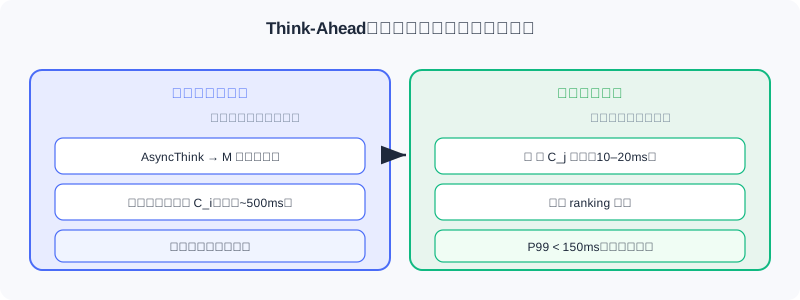
🧠 Mental Model: Everyday Decision-Making Analogy You don't think from scratch every time you make a decision; you accumulate conclusions like "what kinds of movies I like" over time and quickly apply them when deciding. Think-Ahead separates "thinking ahead" from "choosing on the spot," preserving depth of thought while meeting latency.
Think-Ahead has been fully deployed at Kuaishou, with P99 latency around 153ms and app dwell time improved by 0.159%. Compared with the synchronous scheme: P50 latency down 73% (320→86ms), P99 down 68% (480→153ms), reasoning quality retention 98.5%, cache hit rate 92.3%.
💡 Key Insight: In conversational scenarios, OneRec-Think is also context-aware — when the user expresses negative emotion, the model detects the affective signal and shifts recommendations from general interests toward relaxing, positive content. This marks recommendation evolving from "passive response" to "active understanding."
The success of OneRec-Think is a paradigm leap: from "implicit predictor" to "explicit reasoner." But it still depends on hand-designed reasoning templates and tasks — which leads to the autonomous reasoning paradigm of 9.3.
⚠️ Common Mistakes in 9.2
| # | Mistake | Example | Why It's Wrong | Fix |
|---|---|---|---|---|
| 1 | Treating OneRec-Think as a pure generative model | "It's just like OneRec, generating IDs" | It first generates an explicit reasoning chain, then outputs IDs — it's explainable | Remember: reasoning is part of the decision, not decoration |
| 2 | Ignoring "multi-validity" and applying supervised learning directly | Punishing good recommendations absent from labels with 0-1 labels | Recommendation has no single correct answer; this forces the model into conservatism | Use recommendation-specific rewards + GRPO relative advantages |
| 3 | Assuming GRPO needs an absolutely correct answer | "GRPO requires labeling the standard reasoning" | GRPO only compares relative quality within a group; no absolute standard needed | Sample K rollouts per user and compare relative advantages |
| 4 | Forgetting the latency cost of reasoning | Generating the full reasoning chain synchronously online | Hundreds of ms far exceeds the 100ms real-time requirement | Use Think-Ahead asynchronous pre-computation + lightweight selection |
Chapter Summary
📌 Key Takeaways
| Concept | Key Points | Why It Matters |
|---|---|---|
| Three-stage framework | Alignment → activation → enhancement | From "knowing items" to "learning to think" to "refining reasoning" |
| Reasoning scaffolding | Profile (induction) / evaluation (deduction) / end-to-end | Progressively activates explicit reasoning — auditable and explainable |
| Multi-validity + rewards | Four dimensions: cf/sem/coh/feedback | Fits recommendation, which has no single correct answer |
| GRPO | Relative advantages, no absolute standard needed | Allows multiple effective reasoning patterns to coexist |
| Think-Ahead | Asynchronous pre-computation + lightweight online selection | Preserves deep reasoning under real-time latency |
❓ FAQ
Q1: How does OneRec-Think differ from OneRec in 5.3?
A: OneRec directly generates session lists (it generates but doesn't explain); OneRec-Think first generates a structured reasoning chain, then outputs IDs — turning "thinking" into part of the decision, explainable and auditable.
Q2: Why is GRPO better suited to recommendation than "labeling standard answers"?
A: Recommendation is multi-valid — multiple recommendations for the same user can all be reasonable; there is no single standard answer. GRPO samples multiple rollouts per user and compares only relative quality within the group, avoiding mispunishing "good recommendations absent from the labels" as bad.
Q3: Does Think-Ahead sacrifice reasoning quality?
A: Barely — asynchronous pre-computation can use a larger budget (~500ms) to generate deeper reasoning, while online only lightweight selection happens. Measured reasoning quality retention is 98.5%, and P99 stays < 150ms.
🔗 Connections to Later Chapters
- 9.1 (semantic alignment) — the item alignment stage builds directly on 9.1's semantic indices; the model must first "know" before it can "think."
- 9.3 (autonomous reasoning) — OneRec-Think depends on hand-crafted templates; RecZero/RecOne liberate it into autonomous exploration.
- 5.3 (OneRec) — this chapter is the "thinking" upgrade of OneRec's end-to-end generation.
Practice Problems
Work through all problems in order — they get progressively harder. Each has a complete solution you can reveal after trying it yourself.
Problem 9.2.1 — Classifying the Three Stages 🟢 Easy
Assign each training activity below to one of OneRec-Think's three stages (item alignment / reasoning activation / reasoning enhancement):
- (a) Given an ID prefix, generate a description at the corresponding granularity
- (b) Update reasoning paths with GRPO according to relative rewards
- (c) Generate a structured interest summary from user history
- (d) Fuse multimodal embeddings with attention weighting to obtain semantic IDs
💡 Solution (click to reveal)
Approach: Match against the responsibilities of the three stages.
- (a) Item alignment (Item-Textual Alignment)
- (d) Item alignment (hierarchical representation fusion)
- (c) Reasoning activation (user profile reasoning, induction)
- (b) Reasoning enhancement (GRPO reinforcement learning)
Key points:
- Alignment = knowing items; activation = learning to think; enhancement = refining reasoning.
- The order of the three cannot be reversed.
Problem 9.2.2 — Multi-Validity Judgment 🟢 Easy
A user's history shows a love of sci-fi movies. The model recommends a documentary (which the user also likes), but the documentary is not in the training labels (the labels only record the comedy the user actually clicked). What happens under standard 0-1 supervision? Why doesn't it happen with GRPO?
💡 Solution (click to reveal)
Approach: Analyze with the "multi-validity" framework.
Standard supervision: The documentary is not in the labels → punished as an "error" → the model turns conservative, afraid to recommend reasonable content outside the training set.
GRPO: Multiple rollouts are sampled for the same user, comparing rewards relative to the group. If the documentary rollout's reward (combining cf/sem/feedback) exceeds the group average, its relative advantage is positive and it gets reinforced — it doesn't care about being "in the labels," only about being relatively better.
Key points:
- Multi-validity = multiple reasonable recommendations coexist.
- GRPO uses relative advantages to sidestep the "no absolute standard" dilemma.
Problem 9.2.3 — GRPO Relative Advantage Computation 🟡 Medium
For a given user, 4 reasoning rollouts are sampled with rewards . Compute the group average and each rollout's relative advantage , and identify which should be reinforced or suppressed.
💡 Solution (click to reveal)
Approach: Compute the mean first, then subtract term by term.
Group average:
Reinforce: rollouts 1 and 3 (positive relative advantage); suppress: rollouts 2 and 4 (negative).
Key points:
- Absolute magnitude doesn't matter; only the comparison to the group average does.
- GRPO preserves multiple valid reasonings simultaneously (1 and 3 may take different angles).
Problem 9.2.4 — Designing a Think-Ahead Deployment 🔴 Hard
You are designing the Think-Ahead architecture for short-video recommendation. Write out the "input / output / latency budget" for each of the three components — asynchronous pre-computation, online selection, and incremental update — and explain what engineering benefit a 92.3% cache hit rate delivers.
💡 Solution (click to reveal)
Approach: Break it down by the three components.
- Asynchronous pre-computation: input = the user's history after a new action; output = reasoning paths + corresponding candidate sets ; budget ~500ms (background, doesn't block requests).
- Online selection: input = the union of pre-computed candidates + real-time context; output = final recommendation IDs; budget 10–20ms (lightweight ranking).
- Incremental update: input = new behavior; output = appended update or full recomputation; full recomputation only when the profile changes significantly.
Benefit of the 92.3% hit rate: The vast majority of requests use cached reasoning candidates directly, with no need to trigger full recomputation — saving compute while keeping P99 < 150ms — amortizing the cost of "deep thinking" into idle asynchronous periods.
Key points:
- The key idea: move dense reasoning off the critical path.
- High hit rate = online does almost nothing but lightweight selection.
🏆 Challenge: Reasoning Faithfulness Argument
OneRec-Think's reasoning is "generated first" and then recommended, so there is a risk that the reasoning is mere "post-hoc rationalization." Write no more than 200 words explaining which two types of evidence (drawing on the beam-search consistency / interleaved reasoning mentioned in this chapter) you would use to verify that the reasoning genuinely guides the recommendation rather than decorating it.
💡 Hint
Evidence 1: Beam search consistency — apply beam search to intermediate reasoning steps; if the reasoning text stays strongly aligned with the final item (rather than diverging), the reasoning is truly guiding generation. Evidence 2: ID-text interleaved reasoning — if content anchoring of item tokens stably constrains the direction of the textual causal exposition, and swapping the anchor changes the recommendation, then the reasoning chain and generation are coupled rather than independently produced after the fact. This echoes the original claim that "the reasoning process genuinely guides recommendation generation rather than rationalizing after the fact."
Exploring Autonomous Reasoning
📝 Before You Continue: Finish 9.2 on OneRec-Think first — its reasoning capability depends heavily on hand-designed scaffolding and templates. The question this chapter asks is: can we do away with these human designs and let the model learn to think on its own?
OneRec-Think uses a three-stage framework to make the model "think before recommending," but careful readers will notice: its reasoning capability largely depends on human design. Whether it's the predefined prompt templates of the reasoning scaffolding ("analyze user → evaluate candidates → generate recommendation") or the multi-task objectives of item alignment, all were carefully constructed by researchers based on their understanding of the recommendation scenario. It's like handing a student a detailed step-by-step solution template — the student can follow it, but can hardly be said to truly "understand," let alone explore autonomously on entirely new problems.
This dependence creates three deep problems: limited reasoning paths (templates constrain the thinking space), knowledge bottlenecks of the teacher model (human understanding may be biased or incomplete), and scalability challenges (designing a template set per scenario is costly). The root cause is that OneRec-Think is essentially Imitation Learning — learning from human-designed reasoning examples. Genuine intelligence should have the capacity for Exploratory Learning: autonomously discovering strategies through trial and error guided by a goal and feedback. That is the philosophy of Reinforcement Learning (RL).
After reading this chapter, you will be able to:
- Explain why OneRec-Think counts as imitation learning, and the three major limitations of relying on hand-crafted templates
- Describe RecZero's pure reinforcement learning scheme: Think-before-Recommendation template + rule-based reward + GRPO
- Recount RecZero's emergent capabilities: hierarchical reasoning, negative-signal utilization, cross-domain transfer, and more
- Compare the RecOne hybrid paradigm: cold-start SFT (including aligned/misaligned samples) + RL, and how it balances efficiency with performance ceilings
- Work through 4 tiered practice problems and try the "reasoning capability evolution" interactive demo at the end of the chapter
9.3.0 From Imitation to Autonomy: A Paradigm Shift
RecZero marks a significant shift in the reasoning paradigm: from supervised reasoning dependent on human knowledge, toward autonomous reasoning driven by task objectives. It poses a bold question: can a model, without any teacher guidance or reasoning templates, learn how to think purely by interacting with the recommendation environment?
Imagine dropping an LLM that has never seen a recommendation task into a live environment: the system shows the user's history and item metadata, and the model outputs recommendations; after each recommendation it receives a reward signal (e.g., the gap between the recommendation and the true rating). The reward is the model's only learning signal — it doesn't know what "good reasoning" looks like, nor does any example tell it to analyze the user before evaluating items; it must discover on its own which ways of thinking yield higher rewards.
🧠 Mental Model: The Climber and the Safety Framework
The Think-before-Recommendation template is like a generic framework given to a mountaineer: "first observe the terrain, then choose a route, then assess risks, finally act" — it prescribes the steps and their order, but how to observe and which route to choose are entirely up to the climber. RecZero provides enough structure to guide the direction of exploration while leaving enough freedom for the model to discover scenario-specific optimal strategies.
9.3.1 RecZero: Autonomous Reasoning via Pure Reinforcement Learning
Think-before-Recommendation Prompt Construction
Although purely RL-driven, RecZero still gives the model a structured thinking space. The prompt consists of four parts:
The most crucial is , which defines four structured steps:
These correspond to: extracting user interests from history, summarizing the target item's features, assessing user-item matching, and producing a rating prediction. Note — the template defines only the existence and order of the steps; it does not prescribe what to write in each step, which features to attend to, or how to weigh them. All of that is left for the model to explore during RL.
For example, in a book scenario, the model may autonomously discover the "multi-dimensionality of user interests":
<analyze user> The user's history includes biographies of Lincoln and Franklin, a preference for political figures' life stories;
but also Sapiens, a preference for in-depth historical analysis </analyze user>
<analyze item> The Glory and the Dream: a period history of America, balancing portrayals of politicians with narrative of the era </analyze item>
<match> Satisfies both the political-figure and macro-history interests; the depth of writing fits </match>
<rate> 4.5 </rate>
This "consider multiple interest dimensions simultaneously" strategy was not human-designed — it gradually solidified after the model found that "multi-dimensional matching yields higher rewards."
Rule-Based Reward Modeling
RecZero adopts a minimal yet effective reward:
where is the true rating and is the model's prediction in the step. It looks crude, but the key mechanism is: the reward only evaluates the final rating, while the reasoning path and the prediction are jointly generated, so gradients backpropagate through the entire reasoning process. If some way of reasoning systematically leads to more accurate predictions, the model reinforces it.
For example, early in exploration, version A reasons "user likes sci-fi → this book is sci-fi → match → 4 points" (true rating 2, reward -2); later, version B carefully analyzes "user prefers hard sci-fi; this book is sci-fi romance at its core, doesn't fit → 2 points" (reward 0). After repeated comparisons, the model learns that "matching coarse labels alone isn't enough; one must analyze fine-grained preferences in depth" — this metacognition emerged entirely from trial and error, with no one telling it.
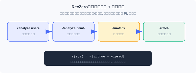
RecZero implements RL with GRPO: for the same sample, sample rollouts , compute relative advantages , reinforcing positive advantages and suppressing negative ones. The model need not know the absolutely correct answer; it only needs to recognize which reasonings are relatively better.
Emergent Capabilities of Pure Reinforcement Learning
After extensive interaction, RecZero exhibits a range of capabilities (not acquired through supervision/imitation, driven purely by reward):
- Hierarchical reasoning forms automatically: from the early minimal "user likes history → match → 4 points," training evolves multi-dimensional profiles and multi-factor trade-offs — the coarse-to-fine evolution is driven entirely by reward signals.
- Utilization of negative signals: the model learns to explicitly note "the user rated horror titles very low; avoid them" — arising from discovering that ignoring explicit dislikes severely lowers the reward.
- Context-sensitive reasoning adjustment: with sparse history (cold start), it falls back to popularity-based conservative predictions; with rich history, it performs deep personalized analysis.
- Cross-domain transfer of reasoning patterns: "distinguishing theme from style" learned in books transfers to "distinguishing story theme from cinematographic style" in movies — evidence that it has learned a general reasoning meta-strategy.
Analysis: The advantage of pure RL is complete autonomy with no teacher bottleneck; the cost is inefficient exploration early in training — discovering effective reasoning patterns from a random state by trial and error is expensive in compute and data. This motivates RecOne's hybrid paradigm.
9.3.2 RecOne: A Cold-Start-Enhanced Hybrid Paradigm
RecZero proved that pure RL lets a model learn to reason autonomously, but exploring "from scratch" is a long and inefficient slog. RecOne's pragmatic compromise: use a small number of high-quality reasoning examples to "cold-start" the model, then let RL refine it autonomously — like "first teaching the basic moves, then letting the student practice and elevate on their own."
Careful Construction of Cold-Start Samples
RecOne's first stage is cold-start supervised fine-tuning (Cold-start SFT), but it differs fundamentally from traditional distillation: only a few high-quality examples are constructed to initialize the reasoning capability. Two strategies:
- Aligned samples: use a pre-trained teacher model to rate user-item pairs; if the prediction happens to match the ground truth, keep the full reasoning path: .
- Misaligned samples: keep samples where the teacher predicted incorrectly, but replace the final step with the correct rating: . This teaches the model "when the line of thought is right but the last step is wrong, distill the useful information and correct it."
The final cold-start set is far smaller than traditional distillation (thousands to tens of thousands vs hundreds of thousands), avoiding overfitting the teacher's surface patterns and leaving ample room for RL optimization. The training objective is standard conditional language modeling .
The Capability Leap from Reinforcement Learning
The second stage is identical to RecZero (GRPO + rating-error reward), but with the cold start in place, the dynamics differ markedly:
- Exploration efficiency leaps: starting from a "can reason" state, exploration focuses on refining and optimizing. Training steps needed to reach the same performance drop by roughly 60%.
- Performance ceiling broken: RecOne ultimately surpasses RecZero by a wide margin — on Amazon-book, RMSE drops 6.7% and MAE 16.8%; on Amazon-music, RMSE drops 12.2% and MAE 29.9%. The reason: RL exploration suffers from local-optimum traps — starting from a random state, it easily converges early to a "decent" simple matching; the cold start provides a starting point closer to the global optimum.
- Diversified reasoning patterns: flexible switching by scenario — fine-grained multi-factor analysis when information is abundant, conservative group-statistics-based reasoning at cold start, exclusion-based reasoning when negative signals are present.
The Essence of the Hybrid Paradigm
RecOne reveals a deep insight: supervised learning and reinforcement learning are not opposites but complements. Supervision provides the "language" (the basic grammatical structure of reasoning); reinforcement provides the "wisdom" (strategy and trade-offs). The human analogy: at school you learn solution steps (supervision); real capability comes from extensive practice and trial and error (reinforcement). The most efficient path is master the basic framework first, then refine through practice. In engineering terms, RecOne's total compute is only 40–50% of RecZero's (small cold-start data, fast RL convergence, avoiding wasteful sampling), making it the better industrial choice.
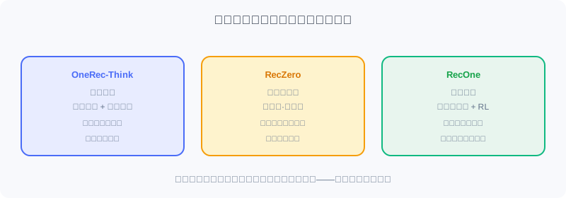
💡 Key Insight: True intelligence is not memorization but reasoning; not imitation but understanding; not following rules but creating strategies. When recommendation acquires autonomous reasoning, it is no longer a passive filter but an active intelligent assistant — understanding deep needs, weighing multi-dimensional objectives, explaining decisions, and continuously learning from feedback.
The interactive demo below recaps the full evolution from "implicit prediction" to "explicit autonomous reasoning":
Click "Next Step" or "Autoplay" and watch how the recommender model departs from the semantic gap, passes through "knowing the items" (LC-Rec/PLUM), "learning to think" (OneRec-Think), and "exploring on its own" (RecZero), and arrives at "hybrid refinement" (RecOne).
⚠️ Common Mistakes in 9.3
| # | Mistake | Example | Why It's Wrong | Fix |
|---|---|---|---|---|
| 1 | Assuming OneRec-Think is already autonomous reasoning | "OneRec-Think explores reasoning autonomously" | It relies on hand-crafted templates/teacher knowledge — essentially imitation learning | Distinguish: imitation (9.2) vs autonomy (RecZero) |
| 2 | Treating the RecZero template as supervision | "The template prescribes what to write at each step" | The template only fixes step order; content is entirely explored by the model | Template = structural guidance, not content supervision |
| 3 | Ignoring the exploration inefficiency of pure RL | Training a large model from scratch with RecZero directly | Massive wasted exploration early on; high cost | Use RecOne cold start + RL for efficiency |
| 4 | Equating cold start with traditional distillation | "RecOne uses millions of teacher samples" | Only thousands to tens of thousands of high-quality (including misaligned) samples | Small but high-quality, leaving room for RL optimization |
Chapter Summary
📌 Key Takeaways
| Concept | Key Points | Why It Matters |
|---|---|---|
| Limits of imitation learning | Template constraints / teacher bottleneck / hard to scale | Motivates autonomous reasoning |
| RecZero pure RL | Framework + free exploration, reward r=−|y−ŷ|, GRPO | Reasoning evolves autonomously without any human knowledge |
| Emergent capabilities | Hierarchical / negative signals / context sensitivity / cross-domain transfer | Proves RL can learn general reasoning meta-strategies |
| RecOne hybrid | Cold-start SFT (aligned + misaligned) + RL | 60% efficiency gain, outperforms RecZero, 40–50% cost |
| Complementary essence | Supervision gives the "language," reinforcement gives the "wisdom" | Framework first, refinement after — the optimal path |
❓ FAQ
Q1: RecZero has no teacher — how does it know whether reasoning is good?
A: It uses only task feedback . The reward evaluates only the final rating, but gradients backpropagate through the whole reasoning — reasoning that is systematically more accurate gets reinforced. No "good reasoning" examples are needed.
Q2: Why does RecOne (with supervised initialization) actually beat pure-RL RecZero?
A: RL exploration has local-optimum traps — from a random state, it easily converges early to simple matching. RecOne's cold start provides a starting point closer to the global optimum, making subsequent exploration more effective, ultimately breaking the performance ceiling with 60% fewer training steps.
Q3: Why are misaligned samples useful?
A: They preserve teacher reasoning that was "right in approach but wrong in the last step," replacing the final rating with the correct value. They teach the model to distill useful information and correct it rather than rejecting the whole line of thought — like a teacher grading homework: "the approach is right, the last step slipped."
🔗 Connections to Later Chapters
- 9.1 (semantic alignment) — all these methods are built on the semantic index representation; autonomous reasoning doesn't change the representation, it changes "how the representation is used to make decisions."
- 9.2 (OneRec-Think) — this chapter is its evolution toward "removing hand-crafted templates": imitation → pure autonomy → hybrid.
- 10.x (diffusion models) — the next chapter switches to a different technical thread — using diffusion's generation/denoising capability for data augmentation and diversity, complementary to the reasoning paradigm.
Practice Problems
Work through all problems in order — they get progressively harder. Each has a complete solution you can reveal after trying it yourself.
Problem 9.3.1 — Paradigm Classification 🟢 Easy
Determine which paradigm each statement describes (imitation learning / pure reinforcement learning / hybrid paradigm):
- (a) Using predefined prompt templates to guide the model through "user profile → candidate evaluation → recommendation"
- (b) No teacher at all; the model explores reasoning autonomously guided only by rating-error rewards
- (c) First SFT on a few high-quality (including misaligned) samples, then autonomous refinement with GRPO
💡 Solution (click to reveal)
Approach: Match against the definitions of the three paradigms.
- (a) Imitation learning (OneRec-Think, hand-crafted templates)
- (b) Pure reinforcement learning (RecZero)
- (c) Hybrid paradigm (RecOne)
Key points:
- Imitation = human knowledge; pure RL = autonomous without knowledge; hybrid = framework first, refinement after.
Problem 9.3.2 — RecZero Reward Computation 🟢 Easy
A rollout predicts rating while the true rating is . Compute RecZero's reward , and explain how the gradient affects the reasoning.
💡 Solution (click to reveal)
Approach: Apply the rule-based reward formula.
Gradient effect: The reward evaluates only the final rating, but the reasoning path and prediction are jointly generated; the negative reward's gradient backpropagates through the whole reasoning, suppressing ways of thinking "that led to overestimation." If another rollout predicts more accurately (higher reward), its reasoning gets reinforced.
Key points:
- The closer the reward to 0 (the more accurate the prediction), the better.
- Good/bad reasoning is reinforced/suppressed respectively via relative advantages.
Problem 9.3.3 — Cold-Start Sample Construction 🟡 Medium
A teacher model predicts rating 4 for a user-item pair whose true rating is also 4 (aligned sample); for another pair it predicts 5 while the true rating is 3 (misprediction). Write out the form each of these two samples takes in RecOne's cold-start set (using the / notation, with explanation).
💡 Solution (click to reveal)
Approach: Classify by the aligned/misaligned definitions.
- Teacher predicts 4 = true 4 → aligned sample: , keep the full reasoning path (because it led to the correct prediction).
- Teacher predicts 5 ≠ true 3 → misaligned sample: , keep the earlier reasoning steps, replacing only with the correct rating 3.
Key points:
- Aligned samples: reasoning → correct answer, kept whole.
- Misaligned samples: wrong answer with a sound approach; fix the last step, teaching the model to distill useful information.
Problem 9.3.4 — Designing Autonomous Reasoning Training 🔴 Hard
You are designing RecOne-style training for music recommendation. Write out: ① which two types of samples the cold-start stage uses and their approximate scale; ② which algorithm and reward the RL stage uses; ③ what gains you expect over using RecZero directly, in terms of "training cost" and "final performance." Cite concrete numbers.
💡 Solution (click to reveal)
Approach: Apply the RecOne hybrid paradigm.
- Cold start: aligned samples (teacher prediction = truth, keep the full reasoning) + misaligned samples (teacher wrong but the final rating step fixed); scale in the thousands to tens of thousands of high-quality samples (far below the millions of traditional distillation).
- RL stage: GRPO, reward , sampling K rollouts per user and comparing relative advantages.
- Gains: training steps down roughly 60% (exploration efficiency); final performance surpasses pure RL — see Amazon-music with RMSE down 12.2% and MAE down 29.9%; total compute at only 40–50% of RecZero's.
Key points:
- Cold start provides the "language"; RL provides the "wisdom."
- The hybrid paradigm both avoids pure RL's inefficiency and breaks through its performance ceiling.
🏆 Challenge: Open-Problem Argument
This chapter notes that autonomous reasoning is still confined to "single-step decisions" (predicting a rating given history and a target item), while real recommendation is "sequential decision-making" (each recommendation affects subsequent behavior and long-term value must be considered). In no more than 200 words, argue: if RecZero were extended to sequential decision-making, how would its reward function need to change? Also identify one "reasoning faithfulness" risk.
💡 Hint
Modification: the single-step immediate-error reward must be replaced by a sequence-level cumulative reward (e.g., long-term interaction value or total session duration over multiple steps), with a discount factor to balance immediate vs long-term value. Risk: reasoning autonomously formed by RL is the product of black-box optimization and may be "post-hoc rationalization" rather than a true reflection of the decision basis, making faithfulness hard to verify — requiring constraints from evidence such as beam-search consistency or interleaved reasoning. This echoes the faithfulness discussion in 9.2 and the open problem at the end of this chapter.
The generative recommendation storyline (see Sections 1.1, 5.3, and 9.x) has shown us that models can "directly generate" item sequences, or even "think before recommending." But generative capability can also solve more practical engineering pain points — data sparsity, missing features, and result homogenization. These are exactly the problems industrial recommender systems have struggled with for years.
Diffusion models offer a unique set of tools for these problems, thanks to their generative paradigm of "gradually adding noise, then learning to remove it." They neither score items like discriminative models nor generate token by token like autoregressive models; instead, they "sculpt" the target in a continuous latent space through multi-step denoising. This part unfolds along two main threads: data augmentation (using diffusion to generate high-quality pseudo-interactions or cross-scenario samples) and feature augmentation and diversity optimization (using diffusion to fill in missing features and generate diverse slates).
What This Part Covers
| Section | Topic | The Big Idea |
|---|---|---|
| 10.1 | Diffusion model basics | Forward noising / reverse denoising, DDPM, latent diffusion, conditional generation and two guidance strategies; special designs for recommendation (noise scale, x₀-prediction) |
| 10.2 | Diffusion for data augmentation | DiffuASR generates "prequel" sequences to extend short-history users; Diff-MSR transfers knowledge across scenarios to ease cold start |
| 10.3 | Diffusion applications in recommendation | AsymDiffRec uses asymmetric diffusion to complete missing features; DMSG uses conditional diffusion to generate diverse slates |
What You'll Be Able to Do After This Part
- 🟢 Explain the two inverse Markov processes of forward diffusion and reverse denoising, and write the direct sampling formula for any t
- 🟢 Distinguish data-space diffusion from latent-space diffusion, and explain why recommendation prefers the latter
- 🟡 Describe the difference between ε-prediction and x₀-prediction, and why recommendation often uses the latter
- 🟡 Recount how DiffuASR / Diff-MSR / AsymDiffRec / DMSG each use diffusion to solve a specific pain point
- 🔴 Critically assess the applicability boundaries of diffusion models in recommendation (latency, supporting infrastructure) and future directions
- Complete the tiered practice problems in each section to consolidate the through-line from basics to deployment
Core Concepts
| Concept | Section | Relevance |
|---|---|---|
| Forward / reverse process | 10.1 | The core inverse mechanism pair of diffusion models |
| Latent diffusion | 10.1 | Recommendation favors LDM due to high dimensionality and sparsity |
| Conditional generation + guidance | 10.1 | Steer generation with user history or text |
| Sequence / cross-scenario augmentation | 10.2 | Eases data sparsity and cold start |
| Asymmetric diffusion / slate generation | 10.3 | Feature completion and diversity optimization |
Prerequisites
- Read Sections 1.1 (two paradigms) and 5.3 (the evolution of the generative paradigm, especially semantic IDs and end-to-end generation)
- Basic probability, variational autoencoders (VAE), and Transformer attention
This part leans toward engineering applications. The math is about "why it is designed this way" — no need to derive every line; just grasp the pain point each method targets.
Tips for This Part
- Always read with the pain point in mind. Each diffusion method maps to a concrete engineering problem (sparsity / cold start / missingness / homogenization).
- Keep the "spaces" straight. Data space vs latent space, forward space vs reverse space — pick the wrong space and the design goes wrong.
- Don't treat diffusion as a replacement for discriminative models. The methods here are tool-style generative capabilities (augmenting data / features / diversity), not an end-to-end replacement for ranking.
Let's dive in! 🚀
Diffusion Model Basics for Recommendation
📝 Before You Continue: Read the two paradigms in 1.1 and the generative paradigm evolution in 5.3 first. This chapter is the "technical groundwork" for deploying diffusion in recommendation; the concrete methods in 10.2/10.3 all build on it.
In 5.3 we discussed, at the architecture level, how diffusion models and Transformers complement each other. This section systematically reviews the core technical principles of diffusion models, with emphasis on the special considerations and design choices when applying them to recommendation. The theoretical foundation comes mainly from DDPM, while DiffRec is the representative work for recommendation applications.
The core idea of diffusion models can be summarized as two inverse Markov processes: forward diffusion gradually adds noise to data, and reverse denoising learns to recover the original data from noise. After reading this section, you will understand this mechanism and why it can serve as a "generative tool" for recommender systems.
After reading this section, you will be able to:
- Write the single-step transition of forward diffusion and the direct sampling formula for any t (reparameterization)
- Distinguish data-space diffusion from latent-space diffusion, and explain why recommendation prefers the latter
- Describe the ELBO training objective and the two parameterizations: ε-prediction and x₀-prediction
- Explain noise scale control in recommendation, inference starting-point selection, conditional generation, and the two guidance strategies
- Complete 4 tiered practice problems, and try the interactive "forward/reverse" demo at the end
10.1.0 Two Operating Spaces of Diffusion Models
By operating space, diffusion models fall into two main families:
Data-space diffusion (pixel-space diffusion) — diffusion and denoising happen directly in the raw data space (image pixels; interaction vectors in recommendation). The representative work is DDPM. It is theoretically more direct, but iterating in a high-dimensional raw space is computationally expensive, and it is especially inefficient for high-resolution data or long sequences.
Latent diffusion models (LDM) — an encoder (VAE / autoencoder) first compresses the raw data into a low-dimensional latent representation space; diffusion and denoising happen there, followed by decoding back to the original space. The representative work is Stable Diffusion. Pipeline: encode → diffuse on → decode . If the dimension drops from to (), the computation can shrink by a factor of .
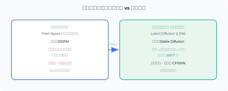
💡 Key Insight: In recommendation, latent diffusion is far more common, for three reasons: ① efficiency — recommendation deals with large-scale behavior sequences and item features, so operating in the raw space is unacceptable; ② semantics — the latent space offers a more compact, semantic representation that fits user interest / item attribute modeling; ③ flexibility — it integrates easily with existing architectures such as CF and GNN. Hence the methods in this part mostly diffuse in item embedding or user feature spaces rather than operating directly on the sparse interaction matrix.
10.1.1 Forward Noising and Reverse Denoising
The Forward Diffusion Process
Given a data sample , the forward process adds Gaussian noise over steps, building latent variables . Each step transitions as:
where controls the noise strength at step . As , approaches a standard Gaussian. Using the reparameterization trick and the additivity of Gaussians, we can sample the noised data at any directly from :
Equivalently:
where and . This allows efficient sampling of any timestep during training, without executing the forward process step by step.
The Reverse Denoising Process
The reverse process starts from and gradually recovers the original data through a learned denoising network. Each denoising step transitions as:
The mean and covariance are parameterized by a neural network; in practice the covariance is often fixed as , and the mean is the focus of learning.
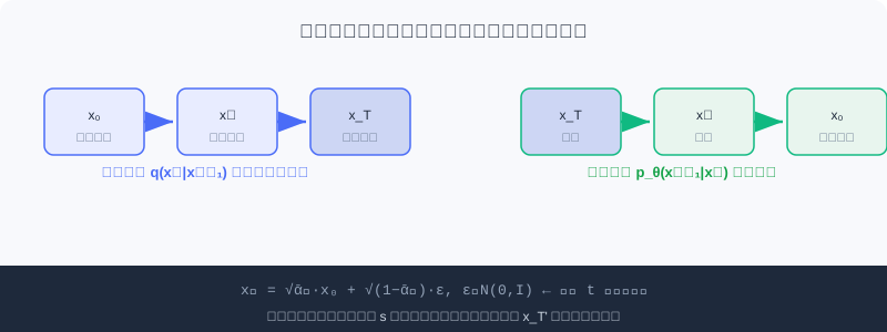
The interactive demo below lets you see how a "user interaction vector" is gradually noised into static and then recovered by denoising:
Click "Next step" or "Autoplay" and watch the signal cells — a clear interaction pattern in the forward pass — get progressively drowned in noise, then recovered by reverse denoising. This is the full process of a diffusion model "sculpting" the target data.
10.1.2 Training Objective and Two Parameterizations
From ELBO to the Simplified Loss
Diffusion models are trained by maximizing the evidence lower bound (ELBO) of the log-likelihood of :
The reconstruction term measures the ability to recover from ; the denoising matching term forces the learned reverse transition to align with the true posterior . At inference time we do not know , so we must train the network to approximate this ideal process.
Two Parameterizations
The denoising network can adopt two parameterizations:
1. Predicting the noise (the DDPM standard):
2. Predicting the original data :
The two are mathematically equivalent (), but recommendation often uses x₀-prediction. The reason: the goal in recommendation is to recover the original interactions from the noised interaction vector and directly use as the interaction prediction score for ranking; moreover, the random noise has high variance, and forcing the network to estimate such an unstable target makes training harder.
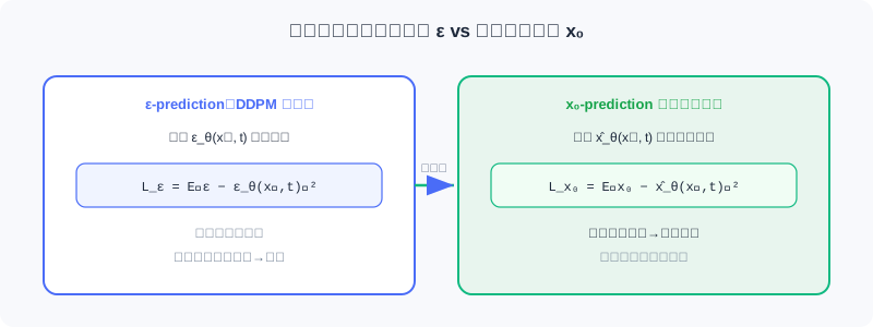
The Sampling Process
After training: ① sample ; ② iterate denoising for :
③ obtain the generated sample .
🧠 Mental Model: The Sculptor and the Block of Stone
Forward diffusion is like gradually hammering an intact marble block into a pile of rubble (noising); reverse denoising is like a sculptor who, guided by an "afterimage," chisel by chisel carves the rubble back into a human figure (denoising). x₀-prediction means the sculptor always imagines directly "what the final figure looks like," which is easier than staring at "the pile of rubble just knocked off" — this is exactly why recommendation prefers it.
10.1.3 Special Designs for Recommendation
Unlike image generation, diffusion in recommendation involves two special designs:
Noise scale control — standard DDPM diffuses data to a pure Gaussian (), but in recommendation completely losing historical preference makes generation harder. So a noise scale parameter limits the maximum strength, keeping part of the original signal even at :
Here controls the upper bound of the overall noise strength, and delimit the interval over which the noise ratio grows linearly with (this design comes from DiffRec and has been widely adopted by subsequent diffusion recommender works).
Inference starting-point selection — inference can start reverse denoising from a partially noised state (), which both leverages denoising to fix noise in the raw interactions and preserves enough personalization information.
Conditional Generation and Controllability
Recommendation wants generation controlled by user history / context. Conditional information can be injected into the denoising network: direct concatenation, additive fusion, or cross-attention in a Transformer. The conditional loss:
At inference, two main strategies steer the generation direction:
1. Classifier-guided — use gradients of a pretrained classifier to push toward the target class:
In recommendation, a sequential recommendation model can serve as the "classifier," guiding generation toward interaction sequences consistent with the history.
2. Classifier-free guidance — during training, replace the condition with an empty placeholder with probability ; at inference:
Large → more personalized but potentially lower quality; small → more diverse but less personalized. More commonly used in recommendation.
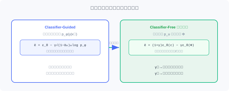
Example conditional design (sequential recommendation): condition on the user's historical interaction sequence, encode it with a Transformer encoder into , and guide diffusion to generate the target item embedding — combining sequence modeling (Transformer) with generative modeling (diffusion). DreamRec adopts exactly this architecture.
Analysis: In recommendation, diffusion does not primarily aim to end-to-end replace discriminative models; instead, its generative capability + random sampling provides tools for two concrete problems: data sparsity and recommendation diversity. This is the through-line for understanding 10.2/10.3.
⚠️ Common Mistakes in 10.1
| # | Mistake | Example | Why It's Wrong | Fix |
|---|---|---|---|---|
| 1 | Diffusing directly on the raw interaction matrix | "Apply DDPM noise to the sparse matrix" | High-dimensional and sparse; computationally unacceptable | Use latent diffusion (LDM) |
| 2 | Forcing ε-prediction into recommendation | "Diffusion recommenders predict noise by default" | Recommendation must recover x₀ and rank on it; x₀ fits better | Use x₀-prediction and output directly |
| 3 | Ignoring the recommendation noise scale | Diffuse all the way to a pure Gaussian before generating | Loses historical preference; generation gets harder | Use scale s to keep part of the signal |
| 4 | Treating classifier-free guidance as more complex | "All guidance needs an extra classifier" | Classifier-free needs no classifier | Distinguish the two types; recommendation usually uses Free |
Chapter Summary
📌 Key Takeaways
| Concept | Key Points | Why It Matters |
|---|---|---|
| Forward / reverse | q adds noise ↔ p_θ denoises; inverse Markov pair | The core mechanism of diffusion models |
| Latent diffusion | Encode → diffuse → decode; computation drops by (d/d')² | Common in recommendation due to high dimensionality and sparsity |
| Two parameterizations | ε-pred vs x₀-pred (equivalent) | x₀-pred fits recommendation better and is the usual choice |
| Special designs for recommendation | Noise scale s, mid-way starting point | Preserves personalization and eases generation |
| Condition + guidance | Concatenation / cross-attention; two guidance types | Steer generation with history / text |
❓ FAQ
Q1: Why does recommendation prefer latent diffusion over data-space diffusion?
A: Interaction vectors in recommendation are high-dimensional and sparse; iterative denoising in the raw space is computationally unacceptable. The latent space is more compact and semantic, integrates easily with CF/GNN, and meets industrial real-time requirements.
Q2: Why does recommendation often use x₀-prediction?
A: The goal of recommendation is to recover the user's original interactions and rank on ; x₀-pred is more stable and better matched to the task than estimating the high-variance noise ε.
Q3: How should the γ of classifier-free guidance be tuned?
A: Large γ → better adherence to the condition (strong personalization) but potentially lower generation quality / diversity; small γ → more diverse but less personalized. Balance "relevance vs diversity" according to business needs.
🔗 Connections to Later Chapters
- 1.1 / 5.3 (paradigms and generative models) Diffusion is the "continuous-space denoising" branch of the generative family, complementary to autoregressive generation.
- 10.2 (data augmentation) DiffuASR / Diff-MSR apply this section's foundations to generating pseudo-interactions.
- 10.3 (applications) AsymDiffRec / DMSG apply denoising capability to feature completion and diversity.
Practice Problems
Work through all problems in order — they get progressively harder. Each has a complete solution you can reveal after trying it yourself.
Problem 10.1.1 — Direct Sampling Formula 🟢 Easy
Given , at step we have and sampled noise . Write the expression for and state the relative magnitudes of the signal and noise terms.
💡 Solution (click to reveal)
Approach: Apply the reparameterization formula.
The signal coefficient is and the noise coefficient is . The signal is slightly stronger than the noise (t is small).
Key points:
- The squared coefficients sum to 1, preserving variance.
- Smaller means a larger noise share; larger t approaches pure noise.
Problem 10.1.2 — Choosing the Space 🟢 Easy
For each scenario below, should you prefer data-space or latent-space diffusion? Briefly justify.
- (a) Denoising 1024×1024 high-resolution images
- (b) Recommendation augmentation on a million-dimensional sparse user-item interaction matrix
💡 Solution (click to reveal)
Approach: Judge by dimensionality and efficiency.
- (a) Data-space diffusion (DDPM works directly in pixel space; the classic image setting).
- (b) Latent diffusion (LDM) — diffusing a million-dimensional sparse matrix directly is computationally unacceptable; encode to a low-dimensional latent space first.
Key points:
- High-dimensional / sparse → latent space.
- Recommendation almost always uses LDM.
Problem 10.1.3 — Comparing Parameterizations 🟡 Medium
A diffusion recommender trained with ε-prediction shows large fluctuations in prediction scores and unstable ranking performance. Explain the likely cause, and why switching to x₀-prediction is more appropriate (cite variance and the task objective).
💡 Solution (click to reveal)
Approach: Analyze the difference between the parameterizations.
Cause: ε-prediction forces the network to estimate the added Gaussian noise , but has high variance — an unstable target — which makes the recovered x₀ ranking scores fluctuate.
Switch to x₀-pred: The recommendation goal is to recover the original interactions and directly rank on as interaction prediction scores — the x₀-pred loss directly optimizes this objective and avoids estimating high-variance noise, giving more stable training and a better fit for recommendation.
Key points:
- The two are mathematically equivalent but differ in task fit.
- In recommendation, "recovering x₀ is the scoring" → choose x₀-pred.
Problem 10.1.4 — Designing Conditional Guidance 🔴 Hard
You need to design a conditional diffusion for sequential recommendation: use a Transformer to encode the user history as the condition , guiding diffusion to generate the next item embedding. Write down: ① how the condition is injected into the denoising network (at least two ways); ② the training and inference formulas of classifier-free guidance; ③ whether γ should be larger or smaller if you want "more personalization while accepting slightly lower diversity."
💡 Solution (click to reveal)
Approach: Apply this section's conditional generation and guidance.
- Injection methods: direct concatenation ; or additive fusion (timestep embedding added into each layer); or the denoising network fuses via cross-attention in a Transformer.
- Classifier-free: during training, replace with the empty with probability ; at inference .
- Increase γ → leans more toward the condition (strong personalization) but slightly lower diversity — matching "more personalization, accept slightly lower diversity."
Key points:
- Conditional injection should run through every denoising layer.
- γ is the relevance-vs-diversity knob.
🏆 Challenge: Arguing About Recommendation Latency
Diffusion inference requires multi-step iterative denoising, while industrial recommendation often demands sub-second (hundred-millisecond) latency. In 200 words or fewer, argue: for the two use cases "data augmentation (offline)" and "online ranking," is the latency cost of diffusion acceptable in each? Point out one accelerated sampling technique that 10.3 will use.
💡 Hint
Offline data augmentation (e.g., DiffuASR generating prequel sequences) can tolerate multi-step denoising, so latency hardly matters; online ranking with multi-step iteration per request can hardly meet the bar — hence diffusion is mostly used for offline augmentation/generation, and used cautiously online. Acceleration technique: DDIM (deterministic few-step sampling); DMSG in 10.3 uses it to cut steps from over a thousand to 50, reaching millisecond level. This echoes the latency design in 10.3.
Diffusion-Based Data Augmentation
📝 Before You Continue: Finish the forward/reverse processes, conditional generation, and guidance in 10.1 first — both DiffuASR and Diff-MSR in this section use "denoising generation" as an augmentation tool.
The core challenge facing recommender systems is data sparsity: interaction data follows a naturally long-tailed distribution — a few popular items accumulate massive interactions while the vast majority of items have very few records. For new users (cold start) and low-activity users, scarce history makes preference modeling difficult. Traditional augmentations (random cropping, reordering) produce limited-quality samples and struggle to capture latent interest patterns.
The generative capability of diffusion models offers a new angle: after learning the data distribution, the model can generate high-quality pseudo-interaction sequences to expand the training data. This section covers two representative methods: DiffuASR, which generates "prequel" sequences of a user's history, and Diff-MSR, which leverages cross-scenario knowledge transfer to solve cold start.
After reading this section, you will be able to:
- Describe DiffuASR's three-component framework (forward / reverse / guidance) and the SU-Net's sequence handling
- Explain how rounding maps continuous embeddings back to discrete item IDs
- Recount Diff-MSR's "a dog looks like a cat" cross-scenario transfer intuition and its four-stage pipeline
- Compare the two guidance types (classifier-guided / classifier-free) as applied in DiffuASR
- Complete 4 tiered practice problems to consolidate the through-line of diffusion for data augmentation
10.2.0 Why Use Diffusion for Augmentation
Sequential recommendation predicts the next item by modeling a user's historical interactions, but it faces data sparsity (most user-item pairs have very few interactions) and the long-tail user problem (most users have histories shorter than 10 items, and performance drops sharply). Traditional augmentation struggles to generate pseudo-sequences that are "semantically consistent."
The advantage of diffusion models: they do not merely transform existing samples — they learn the distribution and then generate new samples. The generated pseudo-interactions are semantically consistent with the real history while filling in the missing "prequel" information.
🧠 Mental Model: Writing Missing Memoir Chapters
A short-history user is like a diary whose owner remembers only the last few pages. Rather than photocopying those pages a few times, DiffuASR reads the style and themes of those pages and helps write the preceding pages that might have happened — the new content coheres with the existing diary while making the biography more complete.
10.2.1 Sequence Augmentation: DiffuASR
DiffuASR's core idea: given an original interaction sequence , generate the corresponding "prequel" sequence (interactions the user might have had before ). Concatenating them yields a longer, more complete history for training downstream sequential recommendation models.
Overall Framework
DiffuASR has three key components:
- Forward process — gradually noises the item embeddings of the target augmentation sequence. The data is an embedding matrix , where is the augmentation length and the embedding dimension.
- Reverse process — recovers the embedding sequence from noise, then maps it back to discrete item IDs via rounding:
(cosine similarity; the nearest item is the output). This step turns continuous generation into an interpretable item sequence. 3. Guidance process — ensures the generated sequence is semantically consistent with the original. The guidance signal comes from an aggregated representation of the original sequence, .
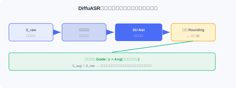
Sequential U-Net
The standard U-Net is designed for images; applying it directly to sequence embeddings loses sequence-dimension information. DiffuASR proposes the SU-Net:
- Treat the sequence dimension as channels: view as an "image" with channels.
- Reshape the embedding dimension: reshape each -dimensional embedding into a matrix.
The input then becomes an -channel, tensor that convolutions handle naturally; each channel is processed independently, preserving sequence position information. The SU-Net body consists of downsampling, intermediate attention layers, and upsampling; the timestep and condition are injected into each ResNet block via additive fusion:
where is the sinusoidal positional encoding of ; is passed through a linear transform and added to each layer's input to steer the denoising direction.
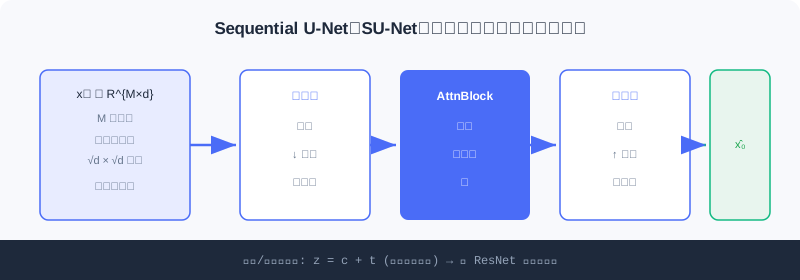
Guidance Strategies
DiffuASR offers two guidance options, corresponding to the two conditional generation methods in 10.1:
1. Classifier-guided — a pretrained sequential recommendation model serves as the "classifier." Since precedes , the first item of can be viewed as the "next item" of ; the guidance objective is to make the generated sequence correctly predict :
2. Classifier-free — randomly drop the condition vector during training, then linearly combine at inference:
This is cleaner and more efficient, and is the more common choice in practice.
Training and Augmentation Pipeline
Training: from the original dataset, select sequences longer than ; the first items serve as the augmentation target and the rest as , with the real prequel supervising the diffusion learning. Augmentation: run guided reverse denoising on each user's sequence to generate a prequel , and concatenate it with the original sequence to form the augmented training data . Sequences generated by DiffuASR can directly train any sequential recommendation model without architectural changes — strong generality.
Analysis: DiffuASR's value lies in "high quality + generality" — the generated pseudo-sequences are semantically consistent and decoupled from the downstream model. The cost: training diffusion + rounding, and generation quality depends on the guidance strength γ.
10.2.2 Cross-Scenario Augmentation: Diff-MSR
In multi-scenario recommendation (MSR), data volume varies drastically across scenarios: popular scenarios have massive interactions, while emerging / vertical (cold-start) scenarios are data-scarce. As a result, cold-start scenario parameters are hard to learn well, and joint training is prone to negative transfer from popular scenarios.
Diff-MSR's insight comes from CV: a blurry photo of a dog may look like a cat. In the recommendation embedding space, user-item embeddings from data-rich scenarios, after appropriate noising, may resemble samples from the cold-start scenario in "outline." This lets us "borrow" knowledge from rich scenarios to augment cold-start ones.
Overall Framework (Four Stages)
- Pretraining — train a multi-scenario backbone (e.g., MMoE) on all-scenario data to obtain a shared embedding layer (cross-scenario general representations).
- Diffusion — for each cold-start scenario, train two diffusion models (positive / negative samples); the input is the concatenation of user feature and item attribute embeddings , learning that scenario's data distribution.
- Classification — train a binary classifier to judge whether a (noised) embedding comes from the cold-start or a rich scenario. Noise rich-scenario samples to varying degrees; those misclassified as cold-start have a similar "outline" and can be exploited.
- Fine-tuning — fine-tune the cold-start model with three kinds of data: pseudo-samples obtained by denoising misclassified rich samples, pseudo-samples generated from pure Gaussian noise, and real cold-start data.
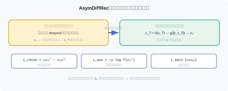
The classification stage is the key: noise a rich-scenario embedding to varying degrees to get ; if it is misclassified as cold-start, this "blurry" sample is similar to the cold-start scenario in embedding space — denoising with the cold-start diffusion model yields a high-quality cold-start sample. Diff-MSR designs a piecewise noise schedule: keep small for the first steps to preserve structure, then grow linearly — light noising still preserves scenario features for classification, while heavy noising ensures convergence to a Gaussian.
💡 Key Insight: The two methods share a common core — use diffusion to generate high-quality pseudo-interaction data, and use conditional control to guarantee semantic consistency. DiffuASR borrows the history condition to generate prequels; Diff-MSR borrows scenario distributions for cross-domain leverage. The next section looks at diffusion applied to features and diversity.
⚠️ Common Mistakes in 10.2
| # | Mistake | Example | Why It's Wrong | Fix |
|---|---|---|---|---|
| 1 | Thinking diffusion augmentation = copying samples | "Copy a short sequence a few times as augmentation" | Copying adds no information and can't fill in prequels | Use diffusion to generate semantically consistent new prequels |
| 2 | Skipping the rounding step | Feed continuous embeddings directly as recommendations | Downstream models need discrete item IDs | Use rounding to map to the nearest item |
| 3 | Confusing the two guidance types | "DiffuASR must use classifier guidance" | Classifier-free is more common and cleaner | Either works; Free is the usual choice |
| 4 | Misusing Diff-MSR across domains | "Cold start can directly use raw rich-scenario samples" | Distributions differ; negative transfer follows | Noise → misclassify → denoise to generate pseudo-samples |
Chapter Summary
📌 Key Takeaways
| Concept | Key Points | Why It Matters |
|---|---|---|
| DiffuASR | Forward / reverse / guidance components + SU-Net + rounding | Generates prequel sequences to extend short-history users |
| SU-Net | Sequence as multi-channel image + additive fusion of condition / timestep | Preserves sequence-dimension information |
| Two guidance types | Classifier / classifier-free | Guarantees semantic consistency with the original |
| Diff-MSR | Four stages + piecewise noise + "dog looks like cat" transfer | Cross-scenario leverage eases cold start |
| Common thread | Generate pseudo-interactions + condition-controlled semantics | Data-augmentation-style diffusion application |
❓ FAQ
Q1: What's the use of the "prequel" generated by DiffuASR?
A: Short-history users lack data, making next-item prediction hard. The semantically consistent prequel concatenates with the original sequence into a longer history, improving downstream sequential recommendation — without coupling to the downstream model.
Q2: Why is rounding necessary?
A: Diffusion denoises in a continuous embedding space, but recommendation needs discrete item IDs to feed downstream models. Rounding takes the nearest item in embedding space, converting continuous results back to interpretable IDs.
Q3: Why does Diff-MSR filter by "misclassification"?
A: If a rich-scenario sample, after noising, is misclassified as cold-start, its outline resembles that scenario — only such samples yield high-quality cold-start pseudo-samples after denoising, avoiding the negative transfer of direct cross-domain use.
🔗 Connections to Later Chapters
- 10.1 (basics) DiffuASR's guidance, the SU-Net's conditional injection, and Diff-MSR's diffusion all build on 10.1's mechanisms.
- 10.3 (applications) shifts from "augmenting data" to "augmenting features and diversity."
- 5.3 / 9.x (generative through-line) Diffusion is the continuous-space branch of the generative family, complementary to autoregressive generation and explicit reasoning.
Practice Problems
Work through all problems in order — they get progressively harder. Each has a complete solution you can reveal after trying it yourself.
Problem 10.2.1 — Framework Classification 🟢 Easy
Assign each component below to one of DiffuASR's three components (forward / reverse / guidance):
- (a) Gradually noising the item embedding matrix
- (b) Using Avg(original sequence embeddings) as the condition c
- (c) Rounding that maps back to discrete item IDs
💡 Solution (click to reveal)
Approach: Check against the three components' responsibilities.
- (a) Forward process
- (b) Guidance process (the condition comes from aggregation of the original sequence)
- (c) Reverse process (rounding after denoising)
Key points:
- Forward = noising; reverse = denoising + rounding; guidance = controlling semantic consistency.
Problem 10.2.2 — Rounding Computation 🟢 Easy
After denoising, the continuous embedding at some position is ; the cosine similarities with three candidates in the item vocabulary are: , , . Which item does rounding select?
💡 Solution (click to reveal)
Approach: Take the candidate with the highest similarity.
The maximum, 0.91, corresponds to → output item A.
Key points:
- Rounding = nearest-neighbor lookup in the vocabulary.
- It "decodes" continuous embeddings into discrete IDs.
Problem 10.2.3 — SU-Net Design 🟡 Medium
What is lost when a standard U-Net is applied directly to sequence embeddings? How does the SU-Net solve this via "sequence as channels" and "embedding reshaping"? Explain how the condition and timestep are injected.
💡 Solution (click to reveal)
Approach: Check against the SU-Net design.
Problem: The U-Net is designed for images; feeding it sequence embeddings directly loses sequence (position) dimension information.
Solution:
- Treat the positions as channels, turning the sequence dimension into the channel dimension;
- Reshape each -dimensional embedding into a matrix, forming an -channel tensor that convolutions can process while each channel (position) is preserved independently.
Injection: the sinusoidal positional encoding of timestep and the condition fuse additively as , then pass through a linear transform and are added to each ResNet block's input to steer the denoising direction.
Key points:
- The core is "preserving the sequence dimension."
- Additive fusion of condition / timestep runs through all layers.
Problem 10.2.4 — Designing Cross-Scenario Augmentation 🔴 Hard
A platform has a "popular e-commerce" scenario and a "newly launched used-car" scenario; the used-car data is extremely sparse. Following the Diff-MSR approach, write the four-stage pipeline, explain why the "piecewise noise schedule" matters, and state which kinds of pseudo-samples are used to fine-tune the cold-start model.
💡 Solution (click to reveal)
Approach: Apply Diff-MSR's four stages.
- Pretraining: train MMoE on all scenarios to get a shared embedding layer.
- Diffusion: train two diffusion models (positive / negative samples) for the used-car scenario; the input is the concatenated user + item attribute embeddings.
- Classification: train a binary classifier to tell whether an embedding comes from used-car or e-commerce; noise e-commerce samples to varying degrees — those misclassified as used-car have a "similar outline" and can be exploited.
- Fine-tuning: use three kinds of data — pseudo-samples from denoising misclassified e-commerce samples, pseudo-samples generated from pure Gaussian noise, and real used-car data.
Why piecewise noise matters: small β early preserves structure so the classifier can judge the "outline"; linear growth later ensures eventual convergence to a Gaussian — otherwise light noising yields no transferable samples, or heavy noising destroys the structure.
Key points:
- "A dog looks like a cat": e-commerce samples noised and misjudged as used-car can be leveraged.
- Pseudo-samples + real data fine-tuned together prevent negative transfer.
🏆 Challenge: Evaluating Augmentation Quality
If the guidance strength γ for DiffuASR is too large, the generated pseudo-sequences may over-fit and lack diversity; too small, and they become semantically inconsistent. In 200 words or fewer, design two computable metrics to evaluate augmentation data quality (one for semantic consistency, one for diversity), and explain how to tune γ accordingly.
💡 Hint
Consistency: similarity between the generated prequel and in embedding space (e.g., average cosine), or the downstream model's accuracy gain on "original + augmented" vs "original only." Diversity: pairwise differences among augmented sequences (e.g., deduplication rate, embedding variance), or the proportion of generated prequels that differ from existing prequels in the training set. γ too large → high consistency but low diversity; γ too small → the reverse; pick a γ at a balance point on the Pareto front of the two.
Feature Augmentation and Diversity Optimization
📝 Before You Continue: Finish 10.1 and 10.2 first — this section's AsymDiffRec and DMSG take the denoising capability beyond "augmenting data" into "augmenting features" and "optimizing outputs."
10.2 used diffusion to generate pseudo-interactions, easing data sparsity and cold start. This section explores the practical value of diffusion from two other angles: feature augmentation and diversity optimization.
In industrial recommendation, missing features are pervasive — incomplete user profiles and absent item attributes directly degrade prediction quality. Meanwhile, traditional deterministic recommendation tends to suggest similar content, and insufficient diversity hurts the experience. Diffusion models offer new approaches to both: denoising is naturally suited to incomplete inputs, and the random sampling mechanism intrinsically supports diversity. This section covers two deployed methods: AsymDiffRec, which uses asymmetric diffusion for feature completion, and DMSG, which uses conditional diffusion to generate diverse recommendation lists.
After reading this section, you will be able to:
- Describe AsymDiffRec's asymmetric design of "discrete forward + latent reverse" and its two losses
- Explain why dropout on discrete features fits real recommendation missingness better than Gaussian noise
- Recount DMSG's slate generation pipeline and its v-prediction parameterization
- Critically assess the applicability boundaries of diffusion in recommendation (latency, supporting infrastructure)
- Complete 4 tiered practice problems
10.3.0 From "Augmenting Data" to "Augmenting Features and Outputs"
Existing diffusion recommenders (such as DiffRec) follow the standard CV recipe: symmetric forward/reverse processes, both using Gaussian noise. But recommendation input features are mostly discrete (user ID, gender, item category); adding continuous Gaussian noise to latent representations of discrete features produces noised representations that do not correspond to any real sample — robustness to Gaussian noise ≠ robustness to the real noise in recommendation. Moreover, the symmetric process may make the model over-attend to noise reconstruction while neglecting personalization information.
💡 Key Insight: Copying diffusion wholesale into recommendation causes a mismatch. Both methods in this section reshape the diffusion process for real recommendation pain points — rather than naively applying the image paradigm. This is the general wisdom for bringing diffusion to recommendation.
🧠 Mental Model: Missing Puzzle Pieces vs a Blurry Photo
Standard diffusion is like adding fog (Gaussian noise) to a "clear photo" — just remove the fog. But missing features in recommendation are more like a puzzle missing a few pieces — not blur, but structural gaps. AsymDiffRec's discrete dropout simulates exactly those "missing pieces," which is closer to reality than adding fog.
10.3.1 Feature Augmentation: AsymDiffRec
AsymDiffRec proposes asymmetric diffusion for two pain points: discrete data-space mismatch (Gaussian noise does not represent real samples) and personalization loss (the symmetric process prioritizes noise over personalization). Its core: the forward process replaces Gaussian noise with discrete feature dropout, the reverse process switches from the raw feature space to the latent representation space, and a task-oriented auxiliary loss preserves personalization.
Discrete Forward Process
Given a sample with features , the forward process performs steps of feature dropout, each randomly dropping one feature, producing the noised sequence . The number of diffusion steps .
The key: after steps, is a sample missing features — highly consistent with online feature missingness (incomplete collection, privacy settings, service failures). So dropout as "noise" matches reality better than Gaussians.
Asymmetric Reverse Process
AsymDiffRec's key innovation: the reverse and forward processes are not in the same space. The forward runs in the raw feature space (dropout); the reverse completes directly in the latent representation space. Let the feature extractor be ; for the noised sample , first extract , and the denoising function takes and the step embedding as input to produce the denoised representation:
The step embedding is a binary vector where marks the corresponding feature as missing, giving the denoiser information about missing positions. Training is driven by a reconstruction loss:
The asymmetry advantage: running the reverse in the raw space (reconstructing missing features, then feeding the extractor) would incur information loss twice (reverse reconstruction + feature extraction); reversing directly in the latent space avoids this — and the latent representation is exactly what recommendation ultimately consumes.
Task-Oriented Auxiliary Loss
Reconstruction loss alone cannot guarantee that personalization is preserved. AsymDiffRec introduces an auxiliary task loss that predicts directly from the denoised representation:
where is a prediction head and is the ground-truth label. This ensures the denoised representation is not only close to the complete representation in L2, but also performs well on downstream prediction.
Training pipeline: ① sample ; ② run the discrete forward to get ; ③ run the asymmetric reverse to get ; ④ jointly optimize .
Inference pipeline: unlike most diffusion recommenders, AsymDiffRec also uses the diffusion module at inference. Online inputs often have missing features; treat them directly as "noised samples," mark the missing positions with the step embedding , and denoise to produce the completed representation . Since the denoising function is a simple two-layer network, the latency impact is minimal.
📊 Data Point: In industrial offline experiments, AsymDiffRec achieved a relative AUC gain of +0.1% and UAUC +1.68%, outperforming CDAE, MultiVAE, self-supervised learning, DiffRec, and others. Ablations show the reconstruction loss and auxiliary task loss are both indispensable — removing the auxiliary loss drops AUC below baseline, showing how critical preserving personalization information is.
10.3.2 Diversity Optimization: DMSG
Scenarios such as music playlists and e-commerce bundles require generating a group of items (a slate) for consumption as a whole, considering coordination among items and overall quality — a combinatorial optimization problem (candidate combinations grow exponentially). Traditional methods assume the user interacts with only one item in the slate (reducing it to single-item recommendation), and deterministic retrieval always returns the same results for the same input, lacking diversity.
DMSG (Diffusion Model for Slate Generation) models slate generation as a conditional generation problem, using diffusion to generate a complete item slate directly from a text prompt. It has three core components:
- Encoding module — converts the discrete item sequence via an embedding function into a continuous representation . It uses a pretrained, frozen encoder that is not jointly trained with the diffusion model, improving stability — and when the catalog updates, only the encoder needs updating.
- Condition module — maps the text prompt to the condition using a Transformer encoding layer, injected into the diffusion via cross-attention.
- Diffusion process module — the core generative module: the forward noises the slate's latent representation, and the reverse recovers it guided by the condition ; the denoising network is a Diffusion Transformer that fuses the condition via cross-attention.
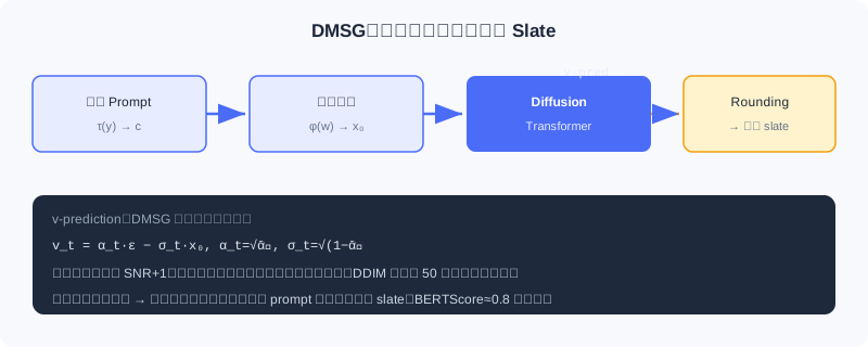
v-prediction Parameterization
10.1 introduced ε-prediction and x₀-prediction; DMSG adopts a third option: v-prediction — predicting the "velocity" , where . From we can recover and . Its advantage: the loss weight is "SNR+1," giving reasonable gradients in both high- and low-SNR regions for more stable training. The loss:
Generation and Decoding
At inference: ① encode the prompt ; ② sample ; ③ iterate conditional denoising; ④ convert the final continuous representation back to a discrete item sequence via rounding (nearest item at each position). To meet latency requirements, DMSG uses DDIM acceleration, cutting inference steps from over a thousand during training down to 50, reaching millisecond-level generation.
Diversity Analysis
DMSG has a natural advantage in diversity, rooted in its random sampling mechanism:
- Item popularity distribution — unlike deterministic retrieval such as BM25, which biases toward high-frequency items, random sampling in the continuous latent space gives low-popularity but semantically relevant items a chance of being selected.
- Freshness of generated results — the same prompt yields different slates on each generation, with comparable quality (BERTScore stable around 0.8) and plenty of new items each time. Users repeatedly requesting the same topic still get different lists, aiding content discovery and retention.
Analysis: AsymDiffRec and DMSG share a common core — reshaping the diffusion process for real recommendation needs instead of applying the image paradigm. The former's asymmetric design solves missing features; the latter's random sampling solves diversity. Both are validated online. Still, diffusion remains some distance from directly replacing discriminative online serving: the latency of multi-step denoising and the supporting infrastructure required for end-to-end generation (e.g., semantic IDs) remain practical constraints on large-scale deployment. The complementarity of diffusion with Transformers, and its fusion with RL / multimodality, remain open directions.
⚠️ Common Mistakes in 10.3
| # | Mistake | Example | Why It's Wrong | Fix |
|---|---|---|---|---|
| 1 | Copying symmetric Gaussian diffusion into recommendation | "Add Gaussian noise and denoise just like images" | Recommendation features are discrete; Gaussians don't represent real missingness | Use AsymDiffRec's discrete dropout |
| 2 | Ignoring personalization loss | Train the diffusion with reconstruction loss only | The model prioritizes noise over personalization; AUC drops | Add the task-oriented auxiliary loss L_aux |
| 3 | Assuming DMSG only uses ε/x₀ prediction | "DMSG just applies DDPM's ε-pred" | DMSG's v-prediction is more stable | Recognize v-pred (SNR+1 weighting) |
| 4 | Overestimating diffusion as a discriminative replacement | "Fully replace ranking with diffusion" | Multi-step denoising latency is high; semantic IDs and other infrastructure required | Treat diffusion as an augmentation tool, not an end-to-end replacement |
Chapter Summary
📌 Key Takeaways
| Concept | Key Points | Why It Matters |
|---|---|---|
| AsymDiffRec | Discrete forward (dropout) + latent reverse + auxiliary loss | Solves industrial missing features; deployed online |
| Asymmetric design | Forward in raw space, reverse in latent space | Avoids double information loss |
| DMSG | Conditional diffusion + v-pred + DDIM | Generates diverse slates; deployed online |
| Source of diversity | Random sampling → long-tail / freshness | Breaks the homogenization of deterministic retrieval |
| Applicability boundary | Latency / supporting infrastructure constrain large-scale deployment | Diffusion is a tool, not an end-to-end replacement |
❓ FAQ
Q1: Why does AsymDiffRec use discrete dropout instead of Gaussian noise?
A: Recommendation features are discrete; Gaussian-noised representations don't correspond to any real sample. Online feature missingness is a "structural gap," and dropout simulates exactly this real missingness — denoising is then completion.
Q2: What's good about DMSG's v-prediction?
A: v = αₜε − σₜx₀; its loss weight is SNR+1, giving reasonable gradients in both high- and low-SNR regions — more stable training than ε/x₀-pred.
Q3: Can diffusion directly replace discriminative ranking?
A: Not yet — multi-step iterative denoising brings latency, and end-to-end generative recommendation requires supporting infrastructure such as semantic IDs. The methods in this part are augmentation tools for data / features / diversity, complementary to Transformers.
🔗 Connections to Later Chapters
- 10.1 (basics) AsymDiffRec's asymmetry and DMSG's v-pred and DDIM all build on 10.1's mechanisms.
- 10.2 (data augmentation) belongs to the same "diffusion as a generative tool" through-line, moving from data → features / outputs.
- 5.3 / 9.x (generative through-line) Diffusion is the continuous-space branch of the generative family, advancing in tandem with autoregressive generation and explicit reasoning.
Practice Problems
Work through all problems in order — they get progressively harder. Each has a complete solution you can reveal after trying yourself.
Problem 10.3.1 — Judging the Asymmetric Design 🟢 Easy
Determine whether each description below belongs to AsymDiffRec's "forward" or "reverse" space:
- (a) Randomly dropping features in the raw feature space
- (b) Denoising in the latent representation space with g([s, z_T])
- (c) The step embedding s marking which features are missing
💡 Solution (click to reveal)
Approach: Check against the asymmetric design.
- (a) Forward (raw feature space, discrete dropout)
- (b) Reverse (latent representation space)
- (c) Reverse (the step embedding is used for denoising in the latent space)
Key points:
- Forward = dropout in raw space; reverse = denoising in latent space.
- Asymmetry means "two stages, two different spaces."
Problem 10.3.2 — The Role of the Auxiliary Loss 🟢 Easy
After removing , AsymDiffRec's AUC even falls below baseline. Explain why.
💡 Solution (click to reveal)
Approach: Analyze from the personalization perspective.
With only the reconstruction loss , the denoised representation is close to the complete representation in L2 distance but may not preserve the personalization information useful for downstream prediction — the model may favor noise reconstruction over personalization. The auxiliary loss forces the denoised representation to also perform well on the prediction task; removing it lets personalization information drain away, and AUC drops below baseline.
Key points:
- Reconstruction ≠ good task performance.
- The auxiliary loss preserves personalization; both losses are indispensable.
Problem 10.3.3 — v-prediction Derivation 🟡 Medium
Given and a predicted , write the formulas recovering and from , and explain the source of v-pred's stability compared to ε-pred.
💡 Solution (click to reveal)
Approach: Apply the v-pred recovery formulas.
Source of stability: v-pred's loss weight is "SNR+1," giving reasonable gradients in both high-SNR (small t) and low-SNR (large t) regions, unlike ε-pred whose gradients become unstable in high-noise regions.
Key points:
- v is a linear combination of ε and x₀ and can be inverted both ways.
- The SNR+1 weighting is the key to its more stable training.
Problem 10.3.4 — Designing Diversity-Oriented Generation 🔴 Hard
You are designing DMSG-style slate generation for a music app. Write down: ① the inputs and outputs of each of the three components (encoding / condition / diffusion); ② why v-prediction and DDIM are used; ③ how to verify the "diversity" improvement (two metrics).
💡 Solution (click to reveal)
Approach: Apply the DMSG design.
- Three components:
- Encoding: item sequence → (frozen pretrained encoder).
- Condition: text prompt → (Transformer encoding).
- Diffusion: guided by condition , a Diffusion Transformer denoises to generate the slate's latent representation.
- Why v-pred: the loss weight is SNR+1, stable across high and low SNR; why DDIM: cuts inference steps from over a thousand to 50, with millisecond-level latency meeting online requirements.
- Diversity verification: ① popularity distribution — compare with BM25 and check whether the share of low-frequency long-tail items rises; ② freshness — generate multiple times from the same prompt and measure the differences across slates (proportion of new items) while quality (BERTScore ≈ 0.8) stays stable.
Key points:
- Random sampling is the intrinsic source of diversity.
- v-pred + DDIM balance stability and latency.
🏆 Challenge: Arguing the Applicability Boundary
This part notes that diffusion "remains some distance from directly replacing discriminative online serving." In 200 words or fewer, list two practical factors constraining large-scale diffusion deployment in recommendation, and propose the fusion direction you find most promising (connecting to the generative through-line of 5.3 / 9.x).
💡 Hint
Constraints: ① the latency cost of multi-step iterative denoising (even DDIM is higher than single-step discriminative models); ② the supporting infrastructure for end-to-end generative recommendation — semantic IDs / quantization — is not yet widespread. Fusion direction: diffusion's denoising generation + Transformer sequence modeling (e.g., DreamRec's conditional diffusion) + reinforcement-learning alignment (echoing GRPO in 9.2), forming a "generation-augmented + controllably aligned" hybrid architecture; or combine with the semantic indexing of 9.x so that diffusion denoises in the semantic ID space.
The preceding chapters covered the core algorithm modules — retrieval, ranking, and re-ranking. But a model that runs in a paper is not the same as a model you can deploy in a real setting — a gap nearly every recommender-system learner runs into. This part uses an end-to-end movie recommender project to string the scattered algorithms into a complete system that runs, serves, and deploys, answering the engineering question: how do you build a production-grade recommender from scratch?
Chapters
| Chapter | Topic | The Big Idea |
|---|---|---|
| 11.1 | Project Introduction and Goals | Clarify the gap between offline evaluation and online deployment; settle the technology choices and the learning path |
| 11.2 | System Architecture Design | Decouple offline from online; the classic funnel of retrieval → ranking → re-ranking |
| 11.3 | Offline Pipeline | Feature engineering, YoutubeDNN/DeepFM training, embedding generation, feature ingestion, and model deployment |
| 11.4 | Online Pipeline | Cold start (UCB), multi-route retrieval (Snake Merge), DeepFM ranking, diversity re-ranking |
| 11.5 | Frontend and Interaction | Five Vue 3 pages, Pinia state, search debouncing, a rating-driven data feedback loop |
| 11.6 | Deployment and Operations | Orchestrate five services with one Docker Compose command; health checks and troubleshooting |
What You Will Be Able to Do After This Part
- 🟢 Describe the responsibility boundary between the offline and online systems, and how the storage layer decouples them
- 🟢 Explain why the funnel architecture is necessary: light models filter candidates in retrieval, heavy models score precisely in ranking
- 🟡 Implement the training loop for YoutubeDNN retrieval and DeepFM ranking, and understand why item embeddings are precomputed
- 🟡 Design a cold-start strategy (UCB exploration + preferred genres + popular fallback) and multi-route retrieval fusion (Snake Merge)
- 🔴 Deploy a multi-container system with PostgreSQL/Redis/Elasticsearch/backend/frontend, and troubleshoot common problems
- 🟢 Complete the tiered practice problems in each section to consolidate the engineering essentials
Key Concepts
| Concept | Section | Relevance |
|---|---|---|
| Offline vs. online | 11.2 | The fundamental boundary of recommender engineering; the quality-vs-latency trade-off |
| Funnel architecture (retrieval → ranking → re-ranking) | 11.2 | The backbone of industrial recommendation |
| Item embedding precomputation | 11.3 | The prerequisite for millisecond-level online vector search |
| Cold start / UCB | 11.4 | The exploration-exploitation balance for new users with no behavior |
| Multi-route retrieval + Snake Merge | 11.4 | Fusion compensates for the coverage gaps of any single strategy |
| Data feedback loop | 11.5 | Frontend behavior feedback drives feature updates and recommendation improvements |
Prerequisites
- The three-stage pipeline mental model from 1.1, and an understanding of how retrieval/ranking/re-ranking divide the work
- The basics of the two-tower model in 2.3 (YoutubeDNN) and the ranking models in 3.x (DeepFM)
- Working knowledge of Python, basic neural networks, and SQL; familiarity with Docker basics is a plus
The code for this project lives in the
web_project/directory of thedatawhalechina/fun-recrepository — you can run it as you read.
Tips for This Part
- Get it running before nitpicking the details. Launch the full project with one Docker Compose command and build overall intuition first.
- Grasp the offline/online boundary. This is the core mental framework for engineered systems.
- Pay attention to the steps papers never mention: how features move across systems, how models update without downtime, and how cold start degrades gracefully.
Let's build it! 🛠️
Project Introduction and Goals
📝 Before You Continue: Finish the three-stage pipeline overview in 1.1 first. This chapter integrates the previously scattered retrieval, ranking, and re-ranking modules into a runnable system — the focus is not on new algorithms, but on making them work together.
Many learners share a very real frustration: they can follow the models in papers and even get the code running, but when asked "how would you deploy a recommender in a real setting?" they have no idea where to start. The gap comes from the distance between offline experimentation and online serving — papers answer "is the model good?" but not "how does the system run?"
After reading this chapter, you will be able to:
- Describe the six fundamental differences between offline evaluation and online deployment
- State this project's four goals: functionally complete, technically realistic, algorithms applied, architecture clear
- List the backend and frontend technology stacks, and explain why FastAPI + Vue + PostgreSQL + Redis + Elasticsearch
- Outline the five-stage learning path from system architecture to deployment
- Work through 4 tiered practice problems to consolidate your picture of the whole project
11.1.0 Project Background: From "Good Model" to "Working System"
The preceding chapters introduced the core modules of a recommender — retrieval, ranking, and re-ranking. They are the building blocks, but how to assemble them into a complete system is something papers don't teach. The real questions you face are:
- When a user opens the app, how does the system return recommendations within 100 milliseconds?
- A user has just rated a movie — how does that behavior immediately affect the next recommendation?
- How are models deployed? Where do features live? How do retrieval and ranking cooperate?
- A brand-new user with no history opens the app for the first time — what should the system recommend?
No single paper answers these questions; you have to think at the system level. This chapter walks you through building a complete movie recommender from scratch: users browse, search, and rate in the browser, backed by a full engineering chain of offline training + online inference + containerized deployment.
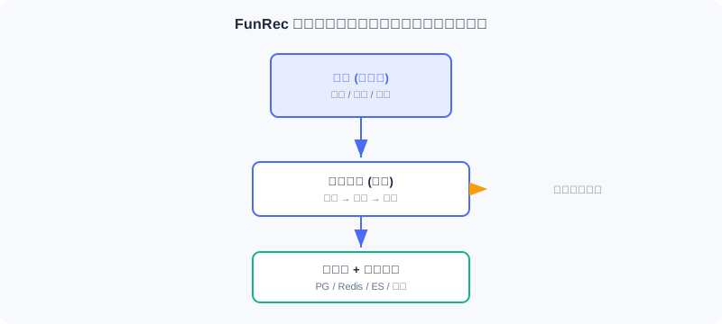
💡 Key Insight: The hard part of engineering practice is not any single algorithm — it is turning discrete modules into a system that runs in concert. Papers give you the parts; this chapter gives you the assembly drawing.
🧠 Mental Model: LEGO Parts vs. a Finished Ship
Reading the algorithm chapters is like collecting LEGO parts — each piece is exquisitely made. But users don't want parts; they want a ship that actually floats and sails. This Part is the process of assembling the parts into a ship — and keeping it afloat for real.
11.1.1 Offline vs. Online
Many readers meet recommender systems through competitions or papers — settings that focus on offline evaluation; this chapter's project focuses on end-to-end deployment — putting a usable system in front of real users. The differences are significant:
| Dimension | Offline Experiments | Online Systems |
|---|---|---|
| Evaluation | Offline metrics (AUC, recall) | Real users actually interacting |
| Data flow | Static datasets | Real-time user behavior |
| Latency requirement | None (batch processing) | Millisecond-level response |
| Cold start | Usually ignored | Must be handled |
| Infrastructure | Local Python scripts | Databases, caches, search engines, container orchestration |
| Final output | Prediction result files | An accessible web application |
The offline system produces at leisure: it processes the full historical data, trains models, and computes embeddings, outputting model files and embedding indexes. The online system serves in real time: it receives requests, invokes models, and assembles results, returning within a few hundred milliseconds. The two are decoupled through the storage layer (Redis, shared files).
Analysis: This decoupling is the pivotal engineering trade-off — offline can chase quality with more complex algorithms and larger data volumes; online only loads the artifacts and focuses on low-latency serving. Understand this boundary, and you understand half of industrial recommender systems.
11.1.2 Technology Choices and Dataset
Dataset: we choose MovieLens-1M — one of the most classic benchmarks in recommendation, with about 1 million ratings, nearly 4,000 movies, and more than 6,000 users. The scale is just right: large enough to exercise the complete architecture, small enough not to blow up your compute budget. We also enrich it with posters, actors, directors, and other metadata from IMDB for a richer display.
Backend stack
- FastAPI: a modern Python web framework, natively async, with auto-generated API docs
- PostgreSQL: the relational store for core business data — users, movies, ratings
- Redis: the in-memory store caching user profiles and real-time behavior sequences
- Elasticsearch: the search engine powering movie search
- Shared file directory: stores the trained models and item embeddings
Frontend stack
- Vue.js 3: a progressive JS framework for building the reactive UI
- Tailwind CSS: a CSS framework for rapid UI implementation
Models and algorithms
- Retrieval: YoutubeDNN two-tower, item-similarity retrieval, user-preferred-genre retrieval
- Ranking: DeepFM (FM second-order crossings + DNN high-order nonlinearity)
- Re-ranking: diversity strategies that scatter by genre and by era
- Cold start / exploration: UCB (Upper Confidence Bound) balancing exploration and exploitation
Infrastructure
- Docker Compose: container orchestration to start all services with one command
- uv: a Python package manager for fast dependency installation
11.1.3 Learning Path
This chapter proceeds from macro to micro, and from offline to online:
- System architecture design (11.2): a top-level view of the components, the offline/online boundary, and how data flows.
- Offline pipeline (11.3): starting from raw data, complete feature engineering, model training, evaluation, and deployment.
- Online pipeline (11.4): build the real-time inference service, implementing cold start, multi-route retrieval, ranking, and re-ranking end to end.
- Frontend and interaction (11.5): design the UI and implement core features such as search, recommendations, and ratings.
- Deployment and operations (11.6): deploy with Docker Compose, and discuss monitoring, logging, and performance tuning.
Every part ships with complete code. You can read and build along, or get the project running first and dig into the details afterwards.
📊 Data Point: All runnable code for this project is in the
web_project/directory of thedatawhalechina/fun-recrepository; the dataset is the preprocessedfunrec-movielens-1m.
⚠️ Common Mistakes in 11.1
| # | Mistake | Example | Why It's Wrong | Fix |
|---|---|---|---|---|
| 1 | Treating offline metrics as launch criteria | "High AUC means it's ready to serve" | Offline has no latency constraint; online must return within a few hundred milliseconds | Distinguish the six dimensions separating offline evaluation from online serving |
| 2 | Ignoring cold start | Assuming every user has history | New users have no behavior; collaborative filtering and vector retrieval fail | Design a dedicated cold-start flow (see Section 11.4) |
| 3 | Over-engineering the stack | Spinning up a K8s cluster for a small project | More operational complexity, slower delivery | One Docker Compose file is enough |
| 4 | Skipping the architecture and diving into code | Writing services before drawing the data flow | Blurry module boundaries, tangled feature hand-offs | Read Section 11.2 first to build the architectural mental model |
Chapter Summary
📌 Key Takeaways
| Concept | Key Points | Why It Matters |
|---|---|---|
| The offline/online gap | Six-dimension differences: evaluation, data, latency, cold start, and more | Papers don't teach it, but engineering must answer it |
| System goals | Functionally complete / technically realistic / algorithms applied / architecture clear | The yardstick for whether a project feels "industrial" |
| Technology stack | FastAPI + Vue + PG + Redis + ES + Compose | Close to industry, reproducible with one command |
| Learning path | Architecture → offline → online → frontend → deployment | Macro to micro, offline to online |
❓ FAQ
Q1: Does this project use generative models, or traditional discriminative ones?
A: The mainline here is a "discriminative three-stage funnel" (YoutubeDNN retrieval + DeepFM ranking + diversity re-ranking) — the classic industrial architecture. It serves as the engineering baseline for the generative recommendation concepts in the later chapters: understanding it is what lets you appreciate what the generative architectures of Chapters 8–10 aim to replace.
Q2: Why not just use one large model to generate recommendations end to end?
A: At this project's scale and latency budget, the funnel architecture is more efficient, controllable, and interpretable. End-to-end generative architectures (see Section 8.2) suit larger scale and more complex needs, but their engineering complexity rises steeply. The two are an evolution, not a replacement.
Q3: Is MovieLens-1M big enough?
A: Enough for teaching and demonstrating the architecture. It runs the full pipeline on a single machine yet contains realistic sparse interactions. Production would use bigger catalogs, but the module boundaries stay the same.
🔗 Connections to Later Chapters
- 1.1 (three-stage pipeline) is the theoretical source of this project's architecture — the funnel structure lands directly here.
- 2.3 (two-tower / YoutubeDNN) and 3.x (DeepFM ranking) provide the algorithmic basis for this project's retrieval and ranking models.
- 11.2 immediately unfolds the system architecture, turning this section's technology choices into components and data flows.
- 8.2 (end-to-end generation) shows the "generative alternative" to this project's architecture, as an advanced contrast.
Practice Problems
Work through all problems in order — they get progressively harder. Each has a complete solution you can reveal after trying it yourself.
Problem 11.1.1 — Offline or Online? 🟢 Easy
Decide whether each description below belongs to the offline system or the online system, and justify your answer:
- (i) Every night, recompute all movie embeddings in a batch job and write them to the shared directory.
- (ii) A user opens the homepage and receives a personalized recommendation list within 200 ms.
💡 Solution (click to reveal)
Answer: (i) Offline system — batch processing, no latency constraint, produces embeddings for the online side to consume. (ii) Online system — real-time request, sub-second latency, serves real users.
Key points:
- Offline optimizes for quality, online for latency; the storage layer decouples them.
- Memorize the six-dimension difference table and you can judge quickly.
Problem 11.1.2 — Matching the Technology Stack 🟢 Easy
Match each requirement to a component of this project: (a) storing user rating records; (b) caching a user's real-time behavior sequence; (c) fuzzy search over movie titles; (d) starting five services with one command.
💡 Solution (click to reveal)
Answer: (a) PostgreSQL; (b) Redis; (c) Elasticsearch; (d) Docker Compose.
Key points:
- Relational data goes to PG, low-latency features to Redis, full-text search to ES, orchestration to Compose.
- Each component solves one well-defined constraint.
Problem 11.1.3 — Why Cold Start Gets Its Own Path 🟡 Medium
A product manager says: "Our retrieval model is accurate — there's no need to handle cold start separately; vector retrieval will recommend just fine." Point out the problem with this claim, and describe how this project deals with it.
💡 Solution (click to reveal)
Answer: Vector retrieval encodes the user vector from historical behavior; a new user has none, so the user vector cannot be built meaningfully and retrieval degrades or fails outright. This project sets up a dedicated cold-start flow: a three-tier strategy of UCB exploration + preference genres set by the user + popular fallback, transitioning to the normal pipeline once behavior accumulates.
Key points:
- Cold start is a structural failure caused by "no behavior" — a better retrieval model cannot cure it.
- Offline evaluation usually ignores cold start, but online must handle it.
🏆 Challenge: Design a Minimal Runnable System 🔴 Hard
If you had to build a movie recommender that "recommends and deploys" with the fewest components, list the core components you would keep (paring down from PG/Redis/ES/FastAPI/Vue/Compose), and justify your choices (within 150 words).
💡 Hint
Minimal set: PostgreSQL (stores data and profiles), FastAPI (retrieval + ranking service), Vue (presentation), Docker Compose (orchestration). Redis and ES can be deferred in the minimal version — features can be read straight from PG (at a latency cost), and search can be replaced by PG fuzzy matching (at a retrieval-quality cost). The essence is closing the loop: request → retrieval → ranking → response.
System Architecture Design
📝 Before You Continue: Finish 11.1 first — the technology choices and the offline/online differences. This section turns those choices into components and data flows, building the top-level mental model of the system.
A production recommender is multiple subsystems working in concert. This section covers the overall design, the core components, and how data moves between them. It is the "map" for all the implementation chapters that follow.
After reading this chapter, you will be able to:
- Describe the responsibility boundary and decoupling between the offline system (production) and the online system (serving)
- Point out the four component groups in the overall architecture diagram: the data storage layer, the offline pipeline, the online pipeline, and the frontend
- Explain the offline data flow (CSV → features/models → shared directory + Redis) and the online data flow (request → retrieval → ranking → re-ranking → assembly)
- Articulate the four key design decisions: the funnel architecture, multi-route retrieval fusion, cold-start handling, and separating feature storage from computation
- Work through 4 tiered practice problems
11.2.0 The Offline and Online Systems
An industrial recommendation architecture splits into two parts: the offline system and the online system.
The offline system is responsible for "production": processing the full historical data, training models, and computing item embeddings and similarity matrices. Compute time is plentiful (hours or even days); it optimizes for model quality rather than response speed, and outputs model files, embedding indexes, feature dictionaries, and the like.
The online system is responsible for "serving": receiving real-time requests, invoking models, assembling recommendation results, and returning them. Response time is limited (sub-second); it must balance quality against latency, and it depends on the models and features the offline side produces.
The offline system runs on a schedule (daily/weekly) and writes its outputs to shared storage; the online system loads from that shared storage. The two are decoupled through the storage layer: offline can afford more complex algorithms and larger data volumes; online focuses on low-latency serving.
The interactive demo below gives you an intuitive feel for how data and models flow between offline "production" and online "consumption": starting from raw rating data, through feature engineering, training, and embedding precomputation, landing in the storage layer, then being loaded by the online service for real-time inference. Click "Next" to watch how each step's outputs get handed off.
Note step five, "storage-layer hand-off": the active.json version pointer and the item embeddings written out by the offline side are exactly the input to the online loading stage — this decoupling is what lets offline retrain at leisure while online serves in milliseconds.
11.2.1 Overall Architecture and Core Components
The system consists of four core component groups, expanded one by one below.
Data Storage Layer
- PostgreSQL (business database): stores the user table (gender/age/occupation), the movie table (title/genres/year/poster), and the ratings table (rating + timestamp).
- Redis (feature cache): holds the real-time features needed for online inference — user profiles
user:{id}:profile, behavior sequencesuser:{id}:history, and the item embedding index. - Shared file directory: stores model files (user_model, ranking_model), the item embedding matrix (item_embeddings.npy), and feature encoding dictionaries (vocab_dict.pkl).
- Elasticsearch (search engine): builds inverted indexes over movie titles, genres, and actors to power search.
Offline Pipeline
Executes in order: feature engineering → retrieval model training (YoutubeDNN) → ranking model training (DeepFM) → model deployment → feature ingestion. See 11.3.
Online Pipeline
Every request passes through: cold-start detection → multi-route retrieval → precise ranking → diversity re-ranking → result assembly. See 11.4.
Frontend Application
Built on Vue 3, with four core pages — home, movie detail, search, and personal center (11.5).
11.2.2 Offline Data Flow
The offline pipeline turns raw rating data into models and features the online side can use:
- Feature engineering: extract training features (user/item/behavior sequences) from the raw ratings.
- Retrieval model training: train the YoutubeDNN two-tower to learn the user/item embedding mapping.
- Ranking model training: train DeepFM to learn the click probability of user-item pairs.
- Model deployment: write the model files to the shared directory for online loading.
- Feature ingestion: write user profiles, behavior sequences, and item information to Redis.
The correspondence between offline outputs and online needs is the key to understanding the whole system — offline "figures out how to compute it," online "fetches it fast and uses it."
11.2.3 Online Data Flow
The online pipeline handles every user request; take "opening the homepage" as an example:
- Cold-start detection: decide whether the user is new (fewer historical behaviors than a threshold); new users go through cold start, everyone else through the normal flow.
- Multi-route retrieval: run YoutubeDNN vector retrieval, item-similarity retrieval, and preferred-genre retrieval in parallel.
- Precise ranking: DeepFM estimates the CTR of each candidate and sorts by score.
- Diversity re-ranking: scattering strategies to avoid consecutive movies of the same genre or year.
- Result assembly: query the database to fill in titles, posters, and so on, and assemble the frontend response.
The target end-to-end latency is under 200 milliseconds.
11.2.4 Key Design Decisions
Separating Retrieval and Ranking (the Funnel Architecture)
In theory you could train one model to score the entire catalog directly, but that is computationally infeasible: with a catalog of 100,000 movies, running the ranking model over the full catalog on every request would take 100 seconds even at 1 ms per inference.
Hence the funnel architecture: the retrieval stage uses a light model to quickly filter down to a few hundred candidates; the ranking stage uses a complex model to score precisely those few hundred.

Multi-Route Retrieval and Fusion (Snake Merge)
Any single retrieval strategy has blind spots: vector retrieval can miss relevance the model never captured; collaborative filtering covers new or niche movies poorly; popular recommendations lack personalization. Fusing multiple strategies lets them cover one another's weaknesses. This project uses Snake Merge: candidates are drawn round-robin from each route, guaranteeing that every route sends representatives into ranking.
Cold-Start Handling
New users lack behavior, so collaborative filtering and vector retrieval fail. This project designs a dedicated cold-start flow: (1) detect via an interaction-count threshold; (2) if the user set preferred genres, prioritize quality movies of those genres; (3) otherwise fall back to popular items or UCB exploration; (4) transition to the normal flow as behavior accumulates.
Separating Feature Storage from Computation
Online inference is latency-sensitive. If every request queried historical behavior from PostgreSQL, the database would become the bottleneck. So high-frequency features are precomputed and written to Redis: user profiles are written at registration/update time; behavior sequences are updated after every rating; item embeddings are written in offline batches. Redis read latency is typically <1 ms — one to two orders of magnitude faster than a database.
Analysis: The four decisions all point to one principle — put the heavy work offline, the fast work online, and the hot data in memory. The funnel solves compute, fusion solves coverage, cold start solves zero samples, and storage separation solves latency.
⚠️ Common Mistakes in 11.2
| # | Mistake | Example | Why It's Wrong | Fix |
|---|---|---|---|---|
| 1 | Scoring the full catalog with one model | "Just rank the whole catalog with one model" | 100k candidates × inference = hundreds of seconds; unservable | Funnel: retrieval narrows the candidates, ranking scores them precisely |
| 2 | Offline/online feature mismatch | Offline uses a new encoder, online the old one | Train-serve skew; performance collapses | Share the same vocab_dict/encoders |
| 3 | Querying the database for features on every request | Reading PG history in real time | The database becomes the latency bottleneck | Pre-write high-frequency features to Redis |
| 4 | Single-route retrieval | Using only vector retrieval | Insufficient coverage; niche/new movies get missed | Multi-route retrieval + Snake Merge fusion |
| 5 | Mixing cold start into the normal flow | Treating new users the same as everyone | Poor experience for new users; recommendations break | Dedicated cold-start detection and a three-tier strategy |
Chapter Summary
📌 Key Takeaways
| Concept | Key Points | Why It Matters |
|---|---|---|
| Offline/online decoupling | Offline produces, online serves; the storage layer bridges them | The engineering balance of quality and latency |
| Four component groups | PG/Redis/shared dir/ES + offline/online/frontend | The physical layout of the system |
| Offline data flow | CSV → features → training → deployment + ingestion | The training-time view |
| Online data flow | Request → retrieval → ranking → re-ranking → assembly | The serving-time view (<200 ms) |
| Four design decisions | Funnel / fusion / cold start / storage separation | The foundation of engineering feasibility |
❓ FAQ
Q1: The offline side runs on a schedule while the online side serves in real time — don't models go stale?
A: They do; that's the norm in industry. This project uses a version pointer (active.json) for transparent hot updates (see Section 11.3): after offline retraining, flipping the pointer is all it takes — no downtime.
Q2: Why are item embeddings computed offline but user embeddings online?
A: The item catalog is relatively static and large — compute it once offline and index it. The user is only known at request time, so their embedding must be computed online. Building the library offline + querying it online is exactly what makes the two-tower scale (see Section 2.3).
Q3: How is Snake Merge different from simply merging by score?
A: Score-based merging lets one route (e.g., vector retrieval) dominate the list; Snake Merge draws round-robin so that every route sends representatives into ranking, improving diversity and coverage.
🔗 Connections to Later Chapters
- 11.1's technology choices land here as components and data flows.
- 11.3 goes deep into every step of the offline pipeline's implementation.
- 11.4 goes deep into every step of the online pipeline's implementation.
- 2.3 (two-tower) and 3.x (DeepFM) are the algorithmic basis of the retrieval and ranking models.
- 4.2 (diversity re-ranking) explains the theoretical motivation for the scattering strategies in the re-ranking stage.
Practice Problems
Work through all problems in order — they get progressively harder. Each has a complete solution you can reveal after trying it yourself.
Problem 11.2.1 — Draw the Data Flow 🟢 Easy
In one sentence: which component produces the offline-trained item_embeddings.npy, which component consumes it, and at which online stage is it used?
💡 Solution (click to reveal)
Answer: The offline pipeline's "model deployment" writes it to the shared directory; the online pipeline's retrieval service (RecallResourceManager) loads it; it is used at the vector-search stage of YoutubeDNN / item-similarity retrieval.
Key points:
- A classic case of offline production and online consumption.
- It embodies "decoupling through the storage layer."
Problem 11.2.2 — The Funnel's Compute Bill 🟢 Easy
A catalog of 50,000 movies; retrieval uses a light model (0.1 ms per candidate) to shortlist 200; ranking uses a heavy model (1 ms per candidate) to score those 200. How long would full-catalog ranking take? How long does the funnel take?
💡 Solution (click to reveal)
Answer: Full-catalog ranking = 50,000 × 1 ms = 50 seconds. Funnel = retrieval 50,000 × 0.1 ms = 5 s + ranking 200 × 1 ms = 0.2 s ≈ 5.2 s. And retrieval over a prebuilt index is far faster than 5 s, so the funnel's advantage is even bigger in practice.
Key points:
- The funnel turns "heavy model over the full catalog" into "light model over the full catalog + heavy model over a subset."
- Real retrieval uses vector indexes and hardly scans the full catalog (see Section 2.3.4).
Problem 11.2.3 — Why Features Live in Redis 🟡 Medium
A product manager argues: "Just query user features straight from PostgreSQL — save yourself the trouble of maintaining Redis." Point out the risks, and quantify why Redis is the better fit.
💡 Solution (click to reveal)
Answer: Every recommendation request reads the user profile + behavior sequence. Querying PG (typically several to a dozen-plus ms per read), stacked on top of retrieval/ranking/re-ranking, easily blows the 200 ms budget; and PG becomes a bottleneck under high concurrency. Redis in-memory reads are <1 ms — one to two orders of magnitude faster than PG — and its List/Hash types naturally express history sequences and profiles. The cost is maintaining one more copy of the data and its consistency, but the latency win far outweighs it.
Key points:
- Online features are "high-frequency, low-latency, structurally simple" → an in-memory store fits naturally.
- PG suits durable business data, not hot-path feature reads.
🏆 Challenge: Propose One Improvement to the Architecture 🔴 Hard
Based on this architecture, propose one change that would noticeably improve recommendation quality or stability in a production environment (e.g., real-time feature updates, model A/B testing, online learning). State the problem it solves and which layer it touches (within 150 words).
💡 Hint
Options: (1) a real-time feature pipeline — update the Redis behavior sequence near-real-time after each rating (instead of only in offline batches) to improve freshness; touches offline "feature ingestion" + an online write-back. (2) Model A/B — extend active.json to multi-version traffic splitting; touches online resource loading. (3) Upgrade vector search to FAISS — replace brute-force inner product once the catalog exceeds a million items; touches the retrieval service. Arguing any one of these is enough.
Offline Pipeline
📝 Before You Continue: Finish 11.2 first — the offline data flow and component boundaries. This section turns those five stages into code: feature engineering → model training → embedding generation → feature ingestion → model deployment.
The offline pipeline carries the recommender's "production" duty, turning raw data into the models and features the online service needs. The whole flow consists of three stages — feature engineering, model training, and storage/deployment — managed through a unified command-line entry that supports running individual steps on demand or the full pipeline.
After reading this chapter, you will be able to:
- Describe the offline directory layout and how
pipeline.pyorchestrates the modules - Build YoutubeDNN sequential samples with a sliding window, and understand the details of left-padding and 1-based encoding
- Explain how the ranking model defines click labels via "relative to the personal mean," and how it mixes hard/random negatives
- Write the code for item embedding precomputation + normalization after YoutubeDNN training, and explain why it matters
- Describe the Redis feature writes (Hash/List + Pipeline) and the model deployment (version pointer) implementations
- Work through 5 tiered practice problems to consolidate the engineering essentials
11.3.0 Code Structure
The offline code lives in web_project/backend/offline/:
offline/
├── pipeline.py # pipeline entry point
├── config.py # configuration management
├── feature/ # feature engineering
│ ├── preprocess_retrieval.py # feature processing for the retrieval model
│ └── preprocess_ranking.py # feature processing for the ranking model
├── training/ # model training
│ ├── train_retrieval.py # retrieval model training
│ └── train_ranking.py # ranking model training
└── storage/ # storage & deployment
├── redis_ingest.py # feature ingestion
└── local_deploy.py # model deployment
The whole flow is orchestrated by pipeline.py, which supports running selected steps on demand:
# offline/pipeline.py
def main():
parser = argparse.ArgumentParser(description="FunRec Offline Pipeline")
parser.add_argument("--steps", type=str, default="all")
args = parser.parse_args()
steps = args.steps.split(",")
if "all" in steps:
steps = ["retrieval_preprocess", "ranking_preprocess",
"retrieval_training", "ranking_training",
"ingest", "deploy"]
if "retrieval_preprocess" in steps:
run_retrieval_preprocessing()
if "ranking_preprocess" in steps:
run_ranking_preprocessing()
if "retrieval_training" in steps:
run_retrieval_training()
if "ranking_training" in steps:
run_ranking_training()
if "ingest" in steps:
ingest_to_redis(flush=args.flush_redis)
if "deploy" in steps:
deploy_local()
This modular design makes debugging easy: you can retrain only the ranking model without touching retrieval. Configuration is centralized in config.py, using environment variables to switch data paths and service addresses:
class Config:
# data paths
TEMP_DIR = Path(os.getenv("FUNREC_PROCESSED_DATA_PATH")) / "web_project"
DATASET_DIR = Path(os.getenv("FUNREC_RAW_DATA_PATH"))
# feature engineering parameters
MAX_SEQ_LEN = 10 # max length of the history sequence
EMB_DIM = 16 # embedding dimension
NEG_SAMPLE_SIZE = 20 # number of negative samples
# training parameters
BATCH_SIZE = 128
EPOCHS = 3
LEARNING_RATE = 0.001
# storage service configuration
DEPLOY_DIR = TEMP_DIR / "deployed_models" # model deployment directory
REDIS_URL = os.getenv("REDIS_URL", "redis://localhost:6379/0")
11.3.1 Feature Engineering
Feature engineering is the most time-consuming and most critical part. Good features boost results dramatically; faulty features often break the model entirely. This project builds samples separately for retrieval and ranking.
Loading the Raw Data
MovieLens-1M has three core tables: users.pkl (6,040 users: gender/age/occupation/zip code), movies.pkl (3,883 movies: title/genres/year), and ratings.pkl (~1 million ratings: user ID/movie ID/rating/timestamp).
def load_raw_data():
df_movies = pd.read_pickle(config.DATASET_DIR / "movies.pkl")
df_ratings = pd.read_pickle(config.DATASET_DIR / "ratings.pkl")
df_users = pd.read_pickle(config.DATASET_DIR / "users.pkl")
return df_movies, df_ratings, df_users
Feature Processing for the Retrieval Model
Categorical feature encoding: recommender features are mostly categorical (user_id, movie_id, gender, genres) and must be encoded as integers to feed an Embedding layer.
def process_features(df_movies, df_ratings, df_users):
user_sparse_feature_columns = ["user_id", "gender", "age", "occupation", "zip_code"]
user_vocab = {}
for feat_name in user_sparse_feature_columns:
label_encoder = LabelEncoder()
new_user_feature_df[feat_name + "_encode"] = (
label_encoder.fit_transform(new_user_feature_df[feat_name]) + 1
) # ← KEY LINE: encodings start at 1; 0 is reserved for unknown/padding
user_vocab[feat_name] = label_encoder.classes_
# the movie side is similar; genres is a list and needs element-wise transform
...
💡 Key Insight: All encoded values start from 1; 0 is reserved for unknowns and padding. Row 0 of the Embedding specifically means "absent/unknown," preventing unknown features from being mistaken for valid IDs.
Behavior sequence construction: the heart of YoutubeDNN is "predict the next movie the user will watch," so samples are built with a sliding window — given the previous watches, predict the -th.
def generate_train_eval_samples(data_df, user_columns, item_columns,
max_hist_seq_len=10, padding_value=0):
data_df.sort_values("timestamp", inplace=True) # ← KEY LINE: sort strictly by time to prevent future leakage
...
for user_id, grouped_feats in data_df.groupby("user_id"):
if len(grouped_feats["movie_id"]) < 2:
continue
len_hist_seq = len(grouped_feats["movie_id"])
# test set: use the last record
...
# training set: sliding window
for i in range(1, len_hist_seq - 1):
train_data_dict["user_id"].append(user_id)
for col in item_columns:
train_data_dict["hist_" + col].append(
add_padding(grouped_feats[col].tolist()[:i],
padding_value, max_hist_seq_len)) # ← KEY LINE: the first i records are the history, record i is the target
train_data_dict[col].append(grouped_feats[col].tolist()[i])
A temporal split simulates the real world: the model may only use past information to predict the future. Random splitting leaks future information — inflated offline metrics, failure online.
Sequence padding: users have different history lengths, but the model needs fixed-length inputs. We use left padding, zero-filling short sequences on the left:
def add_padding(val, padding_value, max_seq_len):
if isinstance(val, (list, tuple, np.ndarray)):
if len(val) > 0 and isinstance(val[0], (list, tuple, np.ndarray)):
val = list(itertools.chain(*val))[-max_seq_len:]
else:
val = list(val)[-max_seq_len:]
return [padding_value] * (max_seq_len - len(val)) + val # ← KEY LINE: pad zeros on the left; the most recent behavior sits on the right
else:
return val
Left padding keeps the most recent behavior on the right side of the sequence — consistent with chronological order and more natural for RNNs/Transformers.
Feature Processing for the Ranking Model
The ranking model (DeepFM) does CTR estimation: given a user-item pair, output a click probability — which requires positive and negative samples.
Label definition: MovieLens has only ratings, no click signal, so labels are defined relative to each user's mean rating:
user_avg_ratings = df_ratings.groupby("user_id")["rating"].mean().reset_index()
df_ratings = df_ratings.merge(user_avg_ratings, on="user_id", how="left")
df_ratings['is_click'] = (
df_ratings['rating'] >= df_ratings['user_avg_rating'] - 1
).astype(int) # ← KEY LINE: ratings at or above (personal mean − 1) count as positive
This approach accounts for differences in rating habits (some people rate high across the board, others harshly); a relative offset reduces individual variance.
Negative sampling: positives come from ratings; negatives must be constructed. Two strategies are mixed:
- Hard negatives: items the user was exposed to but did not interact with positively — "hard" to distinguish.
- Random negatives: sampled randomly from un-interacted items — to expand the volume.
This project uses a 1:3 positive-to-negative ratio (1 hard + 2 random). generate_negative_samples first builds a per-user hard-negative pool, then samples randomly from the un-interacted set. The ratio is a trade-off: too many negatives cause imbalance; too few and the model struggles to discriminate.
Train/test split: again a temporal split:
def split_train_test(df_final, test_ratio=0.2, by_time=True):
if by_time and "timestamp" in df_final.columns:
df_final = df_final.sort_values("timestamp")
split_idx = int(len(df_final) * (1 - test_ratio))
train_df = df_final.iloc[:split_idx]
test_df = df_final.iloc[split_idx:] # ← KEY LINE: earlier samples for training, later samples for testing
else:
from sklearn.model_selection import train_test_split
train_df, test_df = train_test_split(df_final, test_size=test_ratio)
return train_df, test_df
11.3.2 Retrieval Model Training (YoutubeDNN)
Retrieval quickly filters candidates from the full catalog. This project uses the YoutubeDNN two-tower (see 2.3): the user tower encodes users, the item tower encodes items, and the inner product expresses the match.
Model configuration highlights:
model_config_dict = {
"features": {
"emb_dim": 16, "max_seq_len": 10, "task_names": ["movie_id"],
"features": [
{"name": "user_id", "group": ["user_dnn"], "vocab_size": ...},
{"name": "movie_id", "group": ["target_item"], "vocab_size": ...},
{"name": "hist_movie_id", "emb_name": "movie_id", # ← KEY LINE: history and target share the embedding
"group": ["raw_hist_seq"], "combiner": "mean", "vocab_size": ...},
]
},
"training": {
"build_function": "funrec.models.youtubednn.build_youtubednn_model",
"model_params": {"emb_dim": 16, "neg_sample": 20, "dnn_units": [64, 32]},
"loss": "sampledsoftmaxloss", "batch_size": 128, "epochs": 3, # ← KEY LINE: Sampled Softmax handles the large vocabulary
},
}
Three points matter: (1) Embedding sharing — historical movie IDs and the target movie share one table, saving parameters and keeping a single space; (2) sequence aggregation — mean compresses variable-length sequences into a fixed dimension (attention is better but costlier); (3) Sampled Softmax — with 3,000+ items, a full Softmax is too expensive, so the loss is computed only over the sampled positives and negatives.
The training flow is wrapped in run_retrieval_training:
def run_retrieval_training():
train_eval_samples = pickle.load(open(config.TRAIN_DATA_PATH, "rb"))
feature_dict = pickle.load(open(config.FEATURE_DICT_PATH, "rb"))
...
models = train_model(cfg.training, feature_columns, processed_data)
metrics = evaluate_model(models, processed_data, cfg.evaluation, feature_columns)
print(build_metrics_table(metrics))
user_model = models[1]
item_model = models[2]
user_model.save(config.SAVED_MODELS_DIR / "user_model")
item_model.save(config.SAVED_MODELS_DIR / "item_model") # ← KEY LINE: save the user tower and the item tower separately
YoutubeDNN returns three models: the full model, the user tower, and the item tower. Online you need only the user tower (to compute user vectors in real time) plus the precomputed item vectors (produced by the item tower).
Item embedding generation — precompute all item vectors offline:
vocab_dict = pickle.load(open(config.VOCAB_DICT_PATH, "rb"))
all_movie_ids = sorted(list(vocab_dict["movie_id"]))
encoded_ids = np.arange(1, len(all_movie_ids) + 1)
item_inputs = {"movie_id": encoded_ids}
embeddings = item_model.predict(item_inputs, verbose=0)
embeddings = embeddings / np.linalg.norm(embeddings, axis=1, keepdims=True) # ← KEY LINE: normalize so the inner product ≡ cosine similarity
np.save(config.ITEM_EMB_PATH, embeddings)
np.save(config.MOVIE_IDS_PATH, np.array(all_movie_ids))
After normalization the inner product equals cosine similarity, taking values in — intuitive to interpret and easy to threshold.
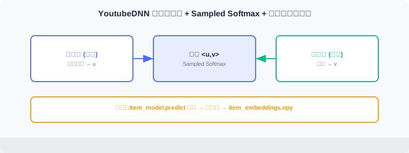
11.3.3 Ranking Model Training (DeepFM)
Ranking scores the retrieval candidates precisely. This project uses DeepFM (see 3.x), combining FM second-order crossings with DNN high-order nonlinearity.
Model configuration needs no tower separation — all features feed the same input:
model_config_dict = {
"features": {
"emb_dim": 16, "task_names": ["is_click"],
"features": [
{"name": "user_id", "group": ["deepfm", "linear"], "vocab_size": ...}, # ← KEY LINE: the same feature feeds both groups
{"name": "movie_id", "group": ["deepfm", "linear"], "vocab_size": ...},
{"name": "genres", "group": ["deepfm", "linear"], "vocab_size": ...},
...
]
},
"training": {
"build_function": "funrec.models.deepfm.build_deepfm_model",
"model_params": {"dnn_units": [128, 64, 32], "dropout_rate": 0.1},
"loss": ["binary_crossentropy"], "metrics": ["binary_accuracy", "AUC"],
"batch_size": 128, "epochs": 3, "validation_split": 0.1,
},
}
The group field assigns each feature: deepfm participates in FM second-order crossings, linear in first-order linear terms. Putting a feature in both lets the model learn both first-order effects and second-order interactions.
The training flow resembles retrieval's, but saves the main model and its configuration (so online inference can reuse the encoders):
def run_ranking_training():
...
models = train_model(cfg.training, feature_columns, processed_data)
main_model = models[0]
metrics = evaluate_model(models, processed_data, cfg.evaluation, feature_columns)
print(build_metrics_table(metrics))
main_model.save(config.RANKING_MODEL_PATH)
pickle.dump({
"feature_dict": feature_dict,
"feature_columns": [fc.name for fc in feature_columns],
"model_config": model_config_dict,
}, open(config.TEMP_DIR / "ranking_model_config.pkl", "wb")) # ← KEY LINE: save the config so the online side can reuse the encoders
Ranking evaluation typically uses AUC (area under the ROC curve), which measures the ability to separate positives from negatives independently of the class balance — reflecting the ability to rank what a user likes higher.
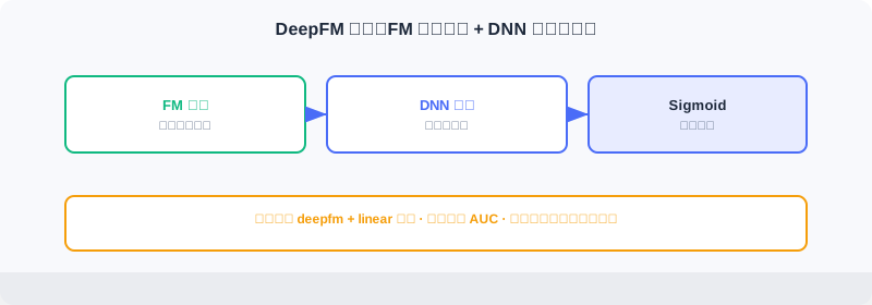
11.3.4 Feature Ingestion and Model Deployment
After training, the outputs must be deployed to storage the online side can reach: Redis for user features, the shared directory for model files.
Writing Features to Redis
def ingest_to_redis(flush: bool = False):
r = redis.Redis.from_url(config.REDIS_URL, decode_responses=True)
if flush:
r.flushdb()
df_movies, df_ratings, df_users = load_raw_data()
pipeline = r.pipeline()
for _, row in df_users.iterrows():
user_id = row['user_id']
key = f"user:{user_id}:profile"
profile_data = {"gender": row["gender"], "age": row["age"],
"occupation": row["occupation"], "zip_code": row["zip_code"]}
pipeline.hset(key, mapping=profile_data) # ← KEY LINE: user profile stored as a Hash
if _ % 1000 == 0:
pipeline.execute() # ← KEY LINE: batch execution to reduce network round trips
pipeline.execute()
# behavior history (List) + preferred genres (top 3, written back to the profile)
df_ratings.sort_values("timestamp", inplace=True)
grouped = df_ratings.groupby("user_id")
for user_id, group in grouped:
history_key = f"user:{user_id}:history"
movie_ids = group["movie_id"].tolist()
pipeline.delete(history_key)
for i in range(0, len(movie_ids), 1000):
chunk = movie_ids[i:i+1000]
pipeline.rpush(history_key, *chunk) # ← KEY LINE: behavior sequence stored as a List, preserving time order
...
top_3 = [g for g, c in Counter(all_genres).most_common(3)]
pipeline.hset(f"user:{user_id}:profile", "frequent_genres", ",".join(top_3))
pipeline.execute()
User profiles use Hashes (key user:{id}:profile), behavior history uses Lists (preserving time order), and the top-3 preferred genres are counted and written back to the profile. Pipeline batching is the key optimization: Redis commands are fast, but every network round trip costs — batching sends significantly speeds up writes.
Local Model Deployment
Model files are large (tens to hundreds of MB) — a poor fit for Redis, so they are managed in the shared directory. The retrieval deployment includes the user-tower model, the item embeddings, and the vocabularies, with an active.json version pointer supporting hot updates:
def deploy_recall_models(deploy_dir: Path):
recall_dir = deploy_dir / "recall"
recall_dir.mkdir(parents=True, exist_ok=True)
shutil.copy2(config.VOCAB_DICT_PATH, recall_dir / "vocab_dict.pkl")
shutil.copy2(config.ITEM_EMB_PATH, recall_dir / "item_embeddings.npy")
user_model_path = config.SAVED_MODELS_DIR / "user_model"
model_deploy_dir = deploy_dir / "model" / "user_recall" / "v1"
model_deploy_dir.mkdir(parents=True, exist_ok=True)
shutil.copytree(user_model_path, model_deploy_dir / "user_model")
version_info = {"version": "v1", "path": "model/user_recall/v1/user_model"}
with open(deploy_dir / "model" / "user_recall" / "active.json", "w") as f:
json.dump(version_info, f) # ← KEY LINE: the version pointer; the online side loads based on it
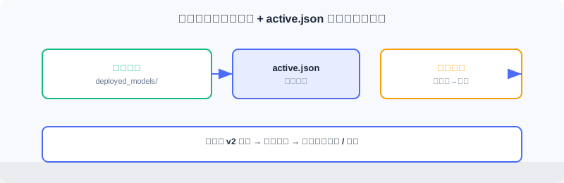
Version management is an essential production capability: through the active.json pointer, the online service knows which version to load; to update, deploy the new version's files first and flip the pointer afterwards — a transparent hot update. Ranking deployment works the same way (writing ranking/active.json).
Analysis: Offline "deployment" is essentially artifact governance — not just training the model right, but landing it in a way the online side can load, hot-update, and roll back. Version pointer + shared directory is a lightweight yet industry-standard approach.
⚠️ Common Mistakes in 11.3
| # | Mistake | Example | Why It's Wrong | Fix |
|---|---|---|---|---|
| 1 | Random split instead of temporal | train_test_split ignoring time | Future leakage — inflated offline, broken online | Split strictly by timestamp |
| 2 | Encoding from 0 | LabelEncoder defaults to 0 | 0 collides with "unknown/padding"; the Embedding misuses it | Add 1 to all encodings; leave 0 for unknowns |
| 3 | Not normalizing item vectors | Saving the raw vectors directly | The inner product isn't cosine; thresholds get arbitrary and interpretation suffers | Normalize offline so the inner product ≡ cosine |
| 4 | All-random negatives | Using only random negatives | No hard examples; the model's discrimination is weak | hard:random = 1:2, overall ratio 1:3 |
| 5 | Deploying without the config | Saving weights but not the encoders/feature columns | Online cannot reproduce the input encoding | Save feature_dict/config pkl alongside |
| 6 | Row-by-row Redis writes | hset in a loop without batching | Network round trips explode; writes crawl | Batch with a pipeline |
Chapter Summary
📌 Key Takeaways
| Concept | Key Points | Why It Matters |
|---|---|---|
| Modular pipeline | pipeline.py orchestrates by step; each runs individually | Easy debugging and incremental updates |
| Sliding-window samples | first predict ; left padding fixes length | Simulates the real "predict the next one" task |
| Temporal split | train/test split by timestamp | Prevents future leakage |
| Item embedding precomputation | offline predict + normalization | Millisecond-level online vector search |
| 1:3 negatives | hard + random mix | Balances discrimination and volume |
| Redis + version pointer | Hash/List + active.json | Fast online reads + transparent hot updates |
❓ FAQ
Q1: Why save the user tower and the item tower separately for retrieval?
A: Online needs only the user tower (real-time user vectors) and the precomputed item vectors (generated offline in batch). The item tower itself isn't used online, but it produces the vectors offline — so both are archived for retraining.
Q2: Why define labels as "personal mean − 1" instead of an absolute threshold?
A: Rating scales differ across users (some live at 4–5, others at 2–3). A relative-to-personal-mean definition treats "high for this person" as positive, removing individual variance and stabilizing labels.
Q3: What does the active.json version pointer solve?
A: The online service reads it at load time to decide the version; after offline retraining you deploy v2 first, then flip the pointer — giving no-downtime hot updates and one-step rollback.
🔗 Connections to Later Chapters
- 2.3 (two-tower) explains the YoutubeDNN structure and Sampled Softmax.
- 3.x (DeepFM) explains the FM+DNN structure and AUC evaluation.
- 11.2 gives the offline data flow and component boundaries.
- 11.4 consumes this section's item vectors, encoders, and models.
- 11.6's offline command
make run-offline-pipelineruns every step of this section.
Practice Problems
Work through all problems in order — they get progressively harder. Each has a complete solution you can reveal after trying it yourself.
Problem 11.3.1 — Why the Temporal Split Matters 🟢 Easy
Why must the ranking model use a temporal rather than a random split? If you used a random split, what would happen to offline AUC versus online performance?
💡 Solution (click to reveal)
Answer: A random split mixes future behavior into training; the model "peeks" at the answers. Offline AUC runs high while online performance collapses (in reality the model can only see the past). A temporal split guarantees that training uses only the past and testing uses the future, so the evaluation tracks online behavior.
Key points:
- Future leakage is a leading cause of the offline-online gap.
- Any recommendation data with timestamps should be split temporally.
Problem 11.3.2 — The Role of Left Padding 🟢 Easy
Why left padding rather than right padding? If a user's history is [A,B,C] (chronological) and MAX_SEQ_LEN=5, what is the sequence after left padding?
💡 Solution (click to reveal)
Answer: Left padding puts the most recent behavior on the right side of the sequence — consistent with time order and more natural for RNNs/Transformers. Padded = [0,0,A,B,C] (two zeros on the left).
Key points:
- 0 is the pad position; the model learns that it carries "no information."
- Recent behavior sits rightmost, so attention/pooling focuses on the recent past.
Problem 11.3.3 — Normalizing Item Vectors 🟡 Medium
After normalization, what is the range of the inner product between user vector and item vector ? Without normalization, what difficulty would threshold-filtering similar candidates run into?
💡 Solution (click to reveal)
Answer: After normalization and the inner product — intuitive to interpret and easy to threshold (e.g., > 0.5). Unnormalized inner products are dominated by vector norms: vectors in the same direction but with different norms can score wildly differently, so no threshold has uniform meaning, and the value cannot double as cosine.
Key points:
- Normalization makes the inner product ≡ cosine similarity.
- Online retrieval (ANN) also depends on this consistency (see Section 2.3.4).
Problem 11.3.4 — The Negative Ratio 🟡 Medium
This project uses a 1:3 positive-to-negative ratio (1 hard + 2 random). If you switched to 1:10 (mostly random), what could go wrong with the model? What about 1:0 (no negatives at all)?
💡 Solution (click to reveal)
Answer: 1:10 leans too hard on easy random negatives; the model only learns to separate "obviously unrelated" pairs, discrimination on hard examples drops, and CTR estimates get coarse. 1:0 means no negatives — Sampled Softmax / binary classification loses its learning signal; the model cannot learn "what is negative" and fails completely.
Key points:
- Negatives are the necessary other half of classification learning.
- Hard negatives sharpen the decision boundary; random negatives supply volume.
🏆 Challenge: Design a Hot Update 🔴 Hard
Suppose the online DeepFM model must be upgraded to v2 — no downtime allowed, and rollback must be possible. Based on the active.json mechanism, describe what the offline side and the online side each need to do (within 150 words).
💡 Hint
Offline: train v2 → deploy to model/ranking/v2/ without touching the pointer yet. Online: the service reads ranking/active.json at load time; to switch, point the pointer at v2 first (hot update) and watch the metrics; if anything goes wrong, point it back at v1 to roll back. The key is "deploy the new files first, flip the pointer second" — the online side only ever reads the pointer, so no restart is needed.
The Online Pipeline
📝 Before You Continue: Read 11.3 first and make sure you understand what the offline stage produces (item embeddings, encoders, user tower / ranking model). This section consumes those artifacts and turns requests into recommendation lists.
The online pipeline must complete the full path from user request to recommendation results within a few hundred milliseconds. The entire flow is encapsulated in a unified recommendation pipeline that executes in the order "cold start detection → multi-route retrieval → precise ranking → diversity re-ranking"; candidate counts and on/off switches for each stage are controlled centrally through configuration.
After reading this chapter, you will be able to:
- Describe how
RecommendationPipelineandPipelineConfigwire the full pipeline together - Explain the cold start detection threshold and the UCB exploration-exploitation formula, and write the score computation and state update code
- Describe the three retrieval routes (YoutubeDNN / I2I / preferred genres) and Snake Merge fusion
- Write DeepFM batch ranking, feature encoding reuse, async execution, and fallback strategies
- Explain how Consecutive Dispersion improves diversity while preserving ordering
- Work through 5 tiered practice problems
11.4.0 Code Structure
The online code lives in web_project/backend/online/:
online/
├── pipeline.py # Main recommendation flow
├── cold_start/ # Cold start handling
│ ├── detector.py # Cold start detection
│ ├── service.py # Cold start service
│ ├── ucb_genre.py # UCB genre exploration
│ └── preferred_genre.py # Preferred-genre strategy
├── recall/ # Multi-route retrieval
│ ├── service.py # Retrieval service and fusion
│ ├── youtubednn.py # YoutubeDNN retrieval
│ ├── item_based.py # Item similarity retrieval
│ └── trending.py # Trending retrieval
├── ranking/ # Ranking models
│ ├── service.py # Ranking service
│ └── deepfm.py # DeepFM ranking
└── reranking/ # Re-ranking strategies
├── service.py # Re-ranking service
└── dispersion.py # Dispersion strategy
The offline artifacts (models in the shared directory, Redis features, item embeddings) are the foundation of the online stage. The online path must finish within 200ms, which demands fast inference, efficient access, and coordinated stages.
The main flow is encapsulated in RecommendationPipeline:
The interactive walkthrough below traces one complete recommendation request: from the moment a user request arrives, through cold start detection, multi-route retrieval, Snake Merge fusion, DeepFM ranking, and diversity re-ranking, to result assembly and return. Click "Next" to watch the candidate pool shrink stage by stage.
Note the candidate counts on the right side of the funnel: the full catalog shrinks to 100 after retrieval and to 20 after ranking, with a target end-to-end latency under 200ms — this is precisely the engineering point of the industrial funnel architecture.
class RecommendationPipeline:
def __init__(self):
self.recall_service = get_recall_service()
self.ranking_service = get_ranking_service()
self.reranking_service = get_reranking_service()
self.cold_start_service = get_cold_start_service()
async def recommend(self, user_features, item_features_provider=None, config=None):
config = config or PipelineConfig()
if config.enable_cold_start and self._is_cold_start(user_features, config):
return await self._cold_start_recommend(user_features, item_features_provider, config)
candidates = await self._recall(user_features, config.recall_top_k)
ranked_items, ranking_strategy = await self._rank(
user_features, candidates, item_features_provider, config.ranking_top_k)
reranked_items, reranking_strategies = await self._rerank(
ranked_items, user_features, item_features_provider)
return RecommendationResult(items=reranked_items, ...)
PipelineConfig centrally controls each stage's behavior:
@dataclass
class PipelineConfig:
recall_top_k: int = 100 # Number of candidates returned by retrieval
ranking_top_k: int = 20 # Number of results returned by ranking
enable_ranking: bool = True # Whether to enable the ranking model
enable_reranking: bool = True # Whether to enable re-ranking
enable_cold_start: bool = True
cold_start_threshold: int = 5 # Fewer interactions than this → cold start user
cold_start_top_k: int = 20
11.4.1 Cold Start Detection and Handling
Cold start is a classic problem: new users have no behavioral data, so both collaborative filtering and embedding-based retrieval fail. This project handles it with a dedicated cold start module.
Cold start detection is straightforward — a user whose interaction history is shorter than the threshold counts as a cold start user:
class ColdStartDetector:
def __init__(self, threshold: int = 5):
self.threshold = threshold
def is_cold_start(self, user_features: Dict[str, Any]) -> bool:
hist_movie_ids = user_features.get("hist_movie_ids", [])
if not hist_movie_ids:
return True
return len(hist_movie_ids) < self.threshold # ← KEY LINE: interaction count < threshold → cold start
The threshold is a trade-off: too low, and users enter the normal flow before their preferences have stabilized; too high, and users wait too long for personalization. The default is 5 interactions.
Three strategies are managed uniformly by ColdStartService:
class ColdStartService:
def __init__(self):
self.detector = ColdStartDetector(threshold=5)
self.strategies = [
UCBGenreStrategy(), # Priority 1: UCB exploration
PreferredGenreStrategy(), # Priority 2: user preferences
PopularRecentStrategy(), # Priority 3: trending fallback
]
async def recommend(self, user_features, top_k=20):
applicable = [s for s in self.strategies if s.can_handle(user_features)]
if has_ucb_data:
allocations = self._get_ucb_weighted_allocation(applicable, top_k)
elif has_preferences:
allocations = self._get_preference_weighted_allocation(applicable, top_k)
else:
allocations = self._get_fallback_allocation(applicable, top_k)
results = await asyncio.gather(*[self._run_strategy(s, user_features, k)
for s, k in allocations if k > 0])
return self._merge_results(results, top_k)
Quotas are allocated dynamically based on user state: with rating history, UCB gets 70%; with only preference settings, the preferred-genre strategy gets 80%; with neither, everything goes to trending.
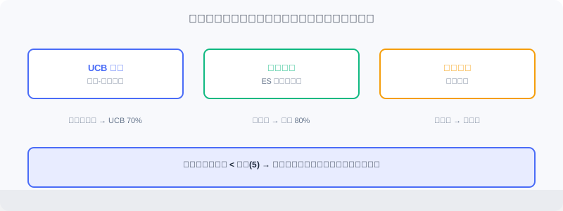
UCB genre exploration solves the exploration-vs-exploitation problem:
where is the historical average rating of genre , is the total number of recommendations, is the number of times genre has been recommended, and is the exploration coefficient. The first term is exploitation (higher average rating is better); the second is exploration (the less a genre has been recommended, the higher the uncertainty and the bonus).
class UCBGenreStrategy(ColdStartStrategy):
def _calculate_ucb_scores(self, stats, total_n):
scores = {}
for genre in self.available_genres:
if genre in stats and stats[genre]["n"] > 0:
n = stats[genre]["n"]
avg_reward = stats[genre]["reward"] / n
exploration_bonus = self.exploration_c * math.sqrt(
math.log(total_n + 1) / (n + 1e-6)) # ← KEY LINE: exploration bonus decays as recommendation count grows
scores[genre] = avg_reward + exploration_bonus
else:
scores[genre] = 1.0 + self.exploration_c * 2 # ← KEY LINE: unexplored genres get the highest exploration score
return scores
UCB statistics are stored in Redis (key user:{user_id}:genre_ucb) and updated whenever the user rates a movie:
def update_ucb_genre_stats(user_id, movie_genres, rating):
normalized_reward = rating / 10.0
key = f"user:{user_id}:genre_ucb"
for genre in movie_genres:
current_raw = redis_client.hget(key, genre)
if current_raw:
current = json.loads(current_raw)
current["n"] = current.get("n", 0) + 1
current["reward"] = current.get("reward", 0) + normalized_reward
else:
current = {"n": 1, "reward": normalized_reward}
redis_client.hset(key, genre, json.dumps(current)) # ← KEY LINE: incrementally update genre statistics
Benefit: as ratings accumulate, the "exploitation" component of UCB grows, while genres the user hasn't encountered still get chances — avoiding the filter bubble.
Preferred-genre strategy: if preferred_genres exists, query Elasticsearch for highly rated movies in those genres (avg_rating>=6.0, rating_count>=20).
11.4.2 Multi-Route Retrieval
Users with enough behavioral history enter the normal flow. The first stage is retrieval: quickly narrow candidates down from the full catalog.
Why multiple routes: any single strategy has blind spots — embedding retrieval can miss relevance the model failed to capture (e.g., newly released niche films with few training samples and inaccurate representations); collaborative filtering undercovers niche items; trending offers no personalization. The idea is "don't put all your eggs in one basket": run several strategies in parallel, then merge.
class RecallService:
def __init__(self):
self.strategies = [
UserPreferenceRecallStrategy(), # User preferred-genre retrieval
ItemEmbeddingRecallStrategy(), # Item similarity retrieval
YouTubeDNNRecallStrategy(), # Embedding retrieval
]
YoutubeDNN embedding retrieval: compute the user embedding online, then retrieve the most similar movies in the item embedding space.
class YouTubeDNNRecallStrategy(RecallStrategy):
def preprocess_user(self, user_features, max_hist_len=10):
inputs = {}
encoders = self.resource_manager.encoders
for feat in ["user_id", "gender", "age", "occupation", "zip_code"]:
raw_val = user_features.get(feat)
if raw_val is not None and feat in encoders:
try:
val = encoders[feat].transform([str(raw_val)])[0] + 1 # ← KEY LINE: reuse the offline encoder, +1 alignment
except:
val = 0
else:
val = 0
inputs[feat] = np.array([val])
# History sequence: encode movie IDs + expand genres, left-pad to fixed length
...
return inputs
def _recall_sync(self, user_context, k):
model_inputs = self.preprocess_user(user_context)
user_emb = self.resource_manager.user_model.predict(model_inputs, verbose=0)
user_emb = user_emb / np.linalg.norm(user_emb, axis=1, keepdims=True)
scores = np.dot(user_emb, self.resource_manager.item_embedding_matrix.T)[0] # ← KEY LINE: inner product ≡ cosine
top_indices = np.argsort(scores)[::-1][:k]
...
Both user and item embeddings are normalized, so the inner product is equivalent to cosine similarity. With a catalog of only 3,000+ items, a direct inner product is fine; beyond a million items, use FAISS to accelerate.
Item similarity retrieval (I2I): recommend items similar to what the user just watched — this captures immediate interests and reuses the YoutubeDNN item embeddings (which themselves encode collaborative filtering signal).
class ItemEmbeddingRecallStrategy(RecallStrategy):
async def recall(self, user_context, k):
hist_movie_ids = user_context.get("hist_movie_ids", [])
if not hist_movie_ids:
return []
last_movie_id = hist_movie_ids[0] # ← KEY LINE: take the most recently watched movie as the seed
enc_idx = movie_le.transform([last_movie_id])[0] + 1
target_emb = self.resource_manager.item_embedding_matrix[enc_idx]
target_emb = target_emb / np.linalg.norm(target_emb)
scores = np.dot(self.resource_manager.item_embedding_matrix, target_emb)
top_indices = np.argsort(scores)[::-1][:k+2]
...
User preferred-genre retrieval: tally the user's preferred genres (computed offline, Top-3 stored in Redis) and retrieve popular movies from those genres. Its strength is stability — even if the user's recent behavior drifts occasionally, it keeps recommending the genres they have liked long-term.
Snake Merge fusion: naively merging by score lets one route dominate the list. Snake Merge takes candidates from the routes in rotation, guaranteeing every route sends representatives into ranking:
def _merge_results_round_robin(self, results_list, top_k):
merged_candidates = []
seen_movie_ids = set()
sources = [r if r else [] for r in results_list]
source_pointers = [0] * len(sources)
direction = 1
current_idx = 0
while len(merged_candidates) < top_k:
all_exhausted = all(source_pointers[i] >= len(sources[i])
for i in range(len(sources)))
if all_exhausted:
break
src_list = sources[current_idx]
ptr = source_pointers[current_idx]
if ptr < len(src_list):
item = src_list[ptr]
source_pointers[current_idx] += 1
mid = item["movie_id"]
if mid not in seen_movie_ids: # ← KEY LINE: deduplicate to avoid cross-route repeats
merged_candidates.append(item)
seen_movie_ids.add(mid)
current_idx += direction
if direction == 1 and current_idx >= len(sources):
direction = -1
current_idx = len(sources) - 1
elif direction == -1 and current_idx < 0:
direction = 1
current_idx = 0
return merged_candidates
The name comes from the traversal order: with three routes A, B, and C, the merge order is A→B→C→C→B→A→A→B→C…, like a snake weaving back and forth.
11.4.3 Precise Ranking (DeepFM)
Retrieval narrows the field to roughly 100 candidates, but their order is determined by retrieval scores and isn't precise enough. Ranking uses DeepFM to estimate CTR for each candidate and reorder them.
The core of online inference is feature construction — each (user, candidate) pair must be encoded into model inputs:
class DeepFMRankingStrategy(RankingStrategy):
def _prepare_batch_inputs(self, user_features, candidates):
rm = self.resource_manager
batch_size = len(candidates)
inputs = {}
for feat in rm.user_features: # ← KEY LINE: user features are shared across all candidates, replicated
raw_val = user_features.get(feat)
encoded_val = rm.encode_feature(feat, raw_val)
inputs[feat] = np.full(batch_size, encoded_val, dtype=np.int32)
for feat in rm.item_features: # ← KEY LINE: item features differ per candidate
encoded_values = [rm.encode_feature(feat, c.get(feat)) for c in candidates]
inputs[feat] = np.array(encoded_values, dtype=np.int32)
return inputs
Feature encoding reuses the LabelEncoders saved offline, with codes starting at 1 and 0 reserved for unknowns, consistent with training:
def encode_feature(self, feat_name, raw_value):
if raw_value is None:
return 0
encoder = self.encoders.get(feat_name)
if encoder is None:
return 0
try:
if isinstance(encoder.classes_[0], str) and not isinstance(raw_value, str):
raw_value = str(raw_value)
if raw_value in encoder.classes_:
return int(encoder.transform([raw_value])[0]) + 1 # ← KEY LINE: strictly consistent with offline encoding
else:
return 0
except Exception:
return 0
Once the inputs are ready, predict in batch:
def _rank_sync(self, user_features, candidates):
inputs = self._prepare_batch_inputs(user_features, candidates)
predictions = self.resource_manager.ranking_model.predict(
inputs, verbose=0, batch_size=min(len(candidates), 256)) # ← KEY LINE: batch prediction exploits vectorization
if predictions.ndim > 1:
predictions = predictions.flatten()
ranked_results = []
for i, candidate in enumerate(candidates):
ranked_results.append({
"movie_id": candidate["movie_id"],
"score": float(predictions[i]), # CTR prediction score
"recall_score": candidate.get("score", 0.0),
"recall_type": candidate.get("recall_type"),
})
ranked_results.sort(key=lambda x: x["score"], reverse=True) # ← KEY LINE: reorder by CTR score
return ranked_results
Batch prediction on 100 candidates typically takes 10–30ms. Model inference is CPU-intensive, so it runs in a thread pool to avoid blocking the event loop; if the model is unavailable, the system falls back to FallbackRankingStrategy, which ranks directly by retrieval score to keep availability high.
11.4.4 Diversity Re-ranking
After retrieval and ranking, the list may lack diversity (e.g., if action movies dominate, ranking pushes them all to the top). Moderate diversity improves satisfaction and retention.
Consecutive Dispersion: no more than consecutive items may share the same attribute. For example, with , [action, action, action, comedy] → [action, action, comedy, action].
class ConsecutiveDispersionStrategy(RerankingStrategy):
def _can_add(self, item, result):
if len(result) < self._max_consecutive:
return True
item_key = self._feature_extractor(item)
if item_key is None:
return True
recent_keys = [self._feature_extractor(r)
for r in result[-(self._max_consecutive - 1):]]
return not all(k == item_key for k in recent_keys) # ← KEY LINE: reject if the last N-1 all match
async def rerank(self, items, user_features=None):
if len(items) <= self._max_consecutive:
return items
result, deferred = [], []
for item in items:
if self._can_add(item, result):
result.append(item)
self._try_insert_deferred(result, deferred) # ← KEY LINE: prefer inserting candidates that can be added
else:
deferred.append(item)
result.extend(deferred) # append the remainder at the end
return result
Two variants are predefined: genre dispersion (uses the first genre) and decade dispersion (buckets by 10-year period, e.g., the 1990s).
class GenreDispersionStrategy(ConsecutiveDispersionStrategy):
def __init__(self, max_consecutive=2):
super().__init__(_extract_genre, max_consecutive, "genre_dispersion")
class DecadeDispersionStrategy(ConsecutiveDispersionStrategy):
def __init__(self, max_consecutive=2):
super().__init__(_extract_decade, max_consecutive, "decade_dispersion")
Strategy chain composition — strategies run in order, each output feeding the next:
class RerankingService:
def __init__(self):
self._strategies = [
GenreDispersionStrategy(max_consecutive=2),
DecadeDispersionStrategy(max_consecutive=2),
]
async def rerank(self, items, user_features=None):
if not items or not self._enabled:
return items
result = items
for strategy in self._strategies:
if strategy.is_ready:
result = await strategy.rerank(result, user_features)
return result
The key property is order preservation: subject to the consecutive constraint, the original order is kept as much as possible — high-scoring items still come first, with only minor positional adjustments — retaining relevance while adding diversity.
11.4.5 API Integration and Service Startup
Once the components are built, they are integrated into FastAPI to expose HTTP endpoints.
Recommendation API core logic:
@router.post("/recommend")
async def get_recommendations(request, db=Depends(get_db), current_user=Depends(get_current_user)):
pipeline = get_pipeline()
if not pipeline.is_ready:
raise HTTPException(status_code=503, detail="Recommendation service not ready")
user_features = await build_user_features(current_user, db)
async def item_features_provider(movie_ids):
movies = await get_movies_by_ids(db, movie_ids)
return {m.id: {"movie_id": m.id, "genres": m.genres.split("|") if m.genres else [],
"year": m.year, "isAdult": m.is_adult} for m in movies}
config = PipelineConfig(recall_top_k=request.recall_top_k or 100,
ranking_top_k=request.top_k or 20, enable_cold_start=True)
result = await pipeline.recommend(user_features=user_features,
item_features_provider=item_features_provider, config=config)
movie_ids = [item.movie_id for item in result.items]
movies = await get_movies_by_ids(db, movie_ids)
movie_map = {m.id: m for m in movies}
return {
"recommendations": [{
"movie_id": item.movie_id, "title": movie_map[item.movie_id].title,
"poster_url": movie_map[item.movie_id].poster_url,
"genres": movie_map[item.movie_id].genres, "year": movie_map[item.movie_id].year,
"score": item.score, "recall_type": item.recall_type,
} for item in result.items if item.movie_id in movie_map],
"is_cold_start": result.is_cold_start, "ranking_strategy": result.ranking_strategy,
}
Key points: (1) user features are assembled from the DB + Redis; (2) the item_features_provider callback lazily loads item features, avoiding loading data at the retrieval stage that may never be used; (3) the pipeline returns IDs + scores, so the database must be queried to fill in titles and posters.
Resource loading and the singleton pattern — models are large and should be shared at process level; RecallResourceManager uses a singleton with lazy loading:
class RecallResourceManager:
_instance = None
def __new__(cls):
if cls._instance is None:
cls._instance = super().__new__(cls)
cls._instance._initialized = False
return cls._instance
def __init__(self):
if self._initialized:
return
self.user_model = None
self.item_embedding_matrix = None
self.encoders = {}
self._initialized = True
def _ensure_resources_loaded(self):
if self.user_model is not None:
return
self._load_from_local() # ← KEY LINE: load only on first use
def _load_from_local(self):
deploy_dir = Path(os.getenv("MODEL_DEPLOY_DIR"))
with open(deploy_dir / "model" / "user_recall" / "active.json") as f:
version_info = json.load(f) # ← KEY LINE: read the version pointer to decide which version to load
self.user_model = tf.keras.models.load_model(deploy_dir / version_info["path"])
self.item_embedding_matrix = np.load(deploy_dir / "item_embeddings.npy")
with open(deploy_dir / "vocab_dict.pkl", "rb") as f:
self.encoders = pickle.load(f)
Health check: /health exposes the status of each component for monitoring:
def get_health_status(self):
return {
"cold_start": {"available": ..., "ready": self.is_cold_start_ready, ...},
"recall": {"available": ..., "strategies": len(self.recall_service.strategies)},
"ranking": {"available": ..., "ready": self.is_ranking_ready, ...},
"reranking": {"available": ..., "ready": self.is_reranking_ready, ...},
}
Analysis: The engineering value of the online path lies in "millisecond latency + high availability" — batch prediction, thread-pool async, model fallback, singleton caching, and hot-loading via version pointers all serve these two goals. These are the details papers never mention, yet they decide whether a system can actually ship.
⚠️ Common Mistakes in 11.4
| # | Mistake | Example | Why It's Wrong | Fix |
|---|---|---|---|---|
| 1 | Encoding inconsistent with offline | Using a default LabelEncoder online | Input space misaligned, predictions are garbage | Reuse the same encoder/vocabulary |
| 2 | Arbitrary cold start threshold | Threshold = 50 | Users wait too long for personalization | Default 5, tune per business |
| 3 | Single retrieval route, no fusion | Only embedding retrieval | Insufficient coverage/diversity | Multi-route + Snake Merge |
| 4 | Ranking without fallback | 503 when the model dies | Availability collapses | FallbackRankingStrategy |
| 5 | Dispersion breaks ordering | Global reshuffle | High scorers pushed back | Preserve order under the consecutive constraint |
| 6 | Reloading the model per request | No singleton | Memory blow-up, high latency | Singleton + lazy loading |
Chapter Summary
📌 Key Takeaways
| Concept | Key Points | Why It Matters |
|---|---|---|
| Pipeline orchestration | Pipeline + Config wire the full flow | Every stage controllable and disableable |
| Cold start UCB | Exploitation + exploration formula, incremental Redis stats | Solves zero-sample exploration-exploitation |
| Multi-route retrieval | Embeddings/I2I/preferences + Snake Merge | Coverage and diversity together |
| Ranking | DeepFM batch CTR estimation + fallback | Precise and highly available |
| Diversity re-ranking | Consecutive dispersion + order preservation | Balances relevance and diversity |
| Resource singleton | Version pointer + lazy loading | Millisecond latency + hot updates |
❓ FAQ
Q1: How was the cold start threshold of 5 chosen?
A: It's an empirical value. Too low, and users enter the normal flow before preferences stabilize (retrieval/ranking are still weak); too high, and users wait too long for personalization. Tune it to your interaction density — lower for high-frequency scenarios, higher for low-frequency ones.
Q2: How is Snake Merge different from naive concatenation with dedup?
A: Naive concatenation sorts by score and truncates to top K, so a strong route can dominate; Snake Merge takes candidates in rotation, structurally guaranteeing every route has representatives entering ranking — better diversity.
Q3: Why not just raise an error when the ranking model dies?
A: Availability comes first in a recommender system. Falling back to ranking by retrieval score still gives users (slightly lower quality) results — far better than a 503. This is the "graceful degradation" principle.
🔗 Connections to Later Chapters
- 11.3 provides item embeddings, encoders, and models — the inputs for all online retrieval/ranking.
- 2.3 (two-tower) and 3.x (DeepFM) are the algorithmic basis of the retrieval and ranking models.
- 4.2 (diversity re-ranking) explains the theoretical motivation for dispersion strategies; this project is an instance of it.
- The recommendation API used in 11.5 calls this section's
pipeline.recommend. - 11.6 discusses how to run this entire online service stably in containers.
Practice Problems
Work through all problems in order — they get progressively harder. Each has a complete solution you can reveal after trying it yourself.
Problem 11.4.1 — Cold Start Determination 🟢 Easy
A user's watch history is [101, 202, 303] (3 movies) and cold_start_threshold=5. What does is_cold_start return? What if they rate 3 more movies (6 total)?
💡 Solution (click to reveal)
Answer: 3 < 5 → returns True (cold start). With 6 total, 6 >= 5 → returns False (normal flow).
Key points:
- The threshold comparison is "fewer than the threshold means cold start."
- Users transition naturally to the normal flow as behavior accumulates.
Problem 11.4.2 — UCB Exploration Term 🟢 Easy
In the UCB formula, genre A has been recommended 100 times and genre B 2 times, everything else equal ( is large). Looking only at the exploration term , which genre scores higher?
💡 Solution (click to reveal)
Answer: B's exploration term = , A's = . The smaller denominator gives the larger value, so B gets the higher exploration bonus. This is exactly "genres recommended less get higher exploration opportunity," avoiding the filter bubble.
Key points:
- The exploration term decreases as grows.
- Unexplored genres (n=0) get the highest exploration score.
Problem 11.4.3 — Snake Merge Order 🟡 Medium
Three retrieval routes A, B, C return candidates [a1,a2], [b1,b2], [c1,c2] respectively, with top_k=4 and no duplicate movie_ids across routes. What are the first 4 items (after dedup) of the Snake Merge result, in order?
💡 Solution (click to reveal)
Answer: The order is A→B→C→C→B→A…. Take a1,b1,c1, then swing back through C for c2. The first 4 = [a1, b1, c1, c2].
Key points:
- The serpentine reverses at the ends, ensuring routes take turns.
- Dedup avoids cross-route duplicates entering ranking.
Problem 11.4.4 — Encoding Consistency 🟡 Medium
The offline LabelEncoder for gender has classes ["F","M"] (transform yields 0/1, +1 gives 1/2). Online, the raw value "M" arrives — what does encode_feature return? What about a value "X" that never appeared in training?
💡 Solution (click to reveal)
Answer: "M" → transform yields 1, +1 returns 2 (consistent with offline). "X" is not in classes_ → returns 0 (unknown), consistent with the offline padding semantics — the model won't crash.
Key points:
- Online must reuse the same offline encoder, with +1 alignment.
- Unknown values uniformly encode to 0, ensuring robustness.
🏆 Challenge: Design a Fallback Chain 🔴 Hard
Suppose that during one request, retrieval works, but the ranking model fails to load, and the user is not a cold start. Describe the path the system should take, the quality of the returned results, and one fallback scheme that could beat "just rank by retrieval score" (within 150 words).
💡 Hint
Path: cold start detection returns False → multi-route retrieval produces candidates → ranking failure triggers FallbackRankingStrategy (sort by retrieval score) → re-ranking → return. Quality: relevance drops (no precise CTR ranking) but stays available. A better scheme: use I2I/preference retrieval scores as coarse-ranking weights, or fall back to a small model that didn't fail (e.g., logistic regression) rather than pure retrieval scores — improving personalization.
Frontend and Interaction
📝 Before You Continue: Read the recommendation API in 11.4 first. This section shows how the frontend calls that API and feeds user behavior back into the system, closing the loop.
The frontend is the user's entry point to the recommender system: browsing, viewing recommendations, searching, rating. These behaviors are collected and fed back to the backend, shaping future recommendations — so the frontend is not just a presentation layer but also a data collection layer.
After reading this chapter, you will be able to:
- List the frontend stack (Vue 3 / Tailwind / Pinia / Vue Router / Axios) and the five core page types
- Implement logged-in/guest access control with route
meta+beforeEachguards - Describe the design essentials of the three core components: MovieCard / MovieRow / StarRating
- Explain how the home page conditionally renders "For You" based on login state and auto-loads recommendations after login
- Manage authentication state centrally with Pinia and control search request frequency with debounce
- Explain how the signup page's preferred genres drive the cold start strategy
- Work through 4 tiered practice problems
11.5.0 Frontend Overview
This project's frontend stack:
| Technology | Purpose |
|---|---|
| Vue.js 3 | Progressive JS framework, uses the Composition API |
| Tailwind CSS | CSS framework, utility classes for fast styling |
| Pinia | State management library, manages auth state |
| Vue Router | Routing, handles page navigation |
| Axios | HTTP client, talks to the backend API |
Core pages: Home (personalized recommendations / trending / categories), Movie Detail (info + rating), Auth (login/signup), Profile (history / preferences), and Search (global real-time search).
💡 Key Insight: The frontend doesn't just "draw the recommendation results" — ratings, views, and searches are collected by the frontend and sent back to the backend, forming the "user behavior → feature update → recommendation improvement" loop. This is what allows the system to keep getting better.
11.5.1 Project Structure and Routing
Directory layout: components/ (reusable), views/ (page-level), services/ (API), stores/ (state).
const routes = [
{ path: '/', name: 'Home', component: Home },
{ path: '/movie/:id', name: 'MovieDetail', component: MovieDetail, props: true },
{ path: '/auth', name: 'Auth', component: Auth, meta: { guest: true } },
{ path: '/profile', name: 'Profile', component: Profile, meta: { requiresAuth: true } },
]
meta flags access requirements, and the navigation guard beforeEach checks them before each transition:
router.beforeEach((to, from, next) => {
const token = localStorage.getItem('token')
if (to.meta.requiresAuth && !token) {
next('/auth') // ← KEY LINE: not logged in → redirect to login
} else if (to.meta.guest && token) {
next('/') // ← KEY LINE: logged-in users can't visit the login page
} else {
next()
}
})
Access logic is centralized in the routing layer; page components don't need to check login state individually.
11.5.2 Core Component Design
MovieCard: the most basic unit. It takes movie and width and displays the poster/title/year/rating. Design essentials: the whole card is a clickable <router-link>; images lazy-load with loading="lazy"; @error listens for load failures and shows a placeholder; group-hover reveals details on hover.
MovieRow: organizes cards into a horizontally scrollable row (Netflix-style). A ref points at the DOM scroll container, and arrows appear dynamically based on scroll position:
import { ref } from 'vue'
const scrollContainer = ref(null)
const showLeftArrow = ref(false)
const showRightArrow = ref(true)
const updateArrows = () => {
const { scrollLeft, scrollWidth, clientWidth } = scrollContainer.value
showLeftArrow.value = scrollLeft > 0
showRightArrow.value = scrollLeft < scrollWidth - clientWidth - 10 // ← KEY LINE: control arrows based on scroll position
}
StarRating: a 10-point star widget. It maintains hoverRating (hovered position) and userRating (saved score); star color follows whichever is active:
const hoverRating = ref(0)
const userRating = ref(0)
const getStarClass = (star) => {
const currentRating = hoverRating.value || userRating.value // ← KEY LINE: hover takes precedence over the saved score
return star <= currentRating ? 'text-yellow-400' : 'text-gray-600'
}
11.5.3 Home Page
The home page consists of a hero banner plus multiple movie rows. Whether to load personalized recommendations depends on login state, watched via watch:
import { ref, watch, onMounted } from 'vue'
import { useAuthStore } from '../stores/auth'
import { movieApi } from '../services/api'
const authStore = useAuthStore()
const forYouMovies = ref([])
const loadingForYou = ref(false)
const fetchRecommendations = async () => {
if (!authStore.isAuthenticated) return
loadingForYou.value = true
try {
const response = await movieApi.getRecommendations(authStore.user.user_id)
forYouMovies.value = response.data
} finally {
loadingForYou.value = false
}
}
watch(() => authStore.isAuthenticated, (isAuthenticated) => {
if (isAuthenticated) {
fetchRecommendations() // ← KEY LINE: auto-load recommendations after login
} else {
forYouMovies.value = [] // ← KEY LINE: clear the list on logout
}
})
Key points: (1) the "For You" row shows only for logged-in users; (2) reactive — auto-load on login, clear on logout; (3) the hero banner prefers the head of personalized recommendations, falling back to trending.
11.5.4 Movie Detail Page
Shows complete information for a single movie. useRoute reads the URL parameter (/movie/123 → route.params.id). Data loading is fault-tolerant: basic info is required, cast is optional:
import { useRoute } from 'vue-router'
const route = useRoute()
const fetchMovieDetails = async () => {
const movieId = route.params.id // ← KEY LINE: get the movie ID from the route
const movieResponse = await movieApi.getMovie(movieId)
movie.value = movieResponse.data
try {
const castResponse = await movieApi.getMovieCast(movieId)
cast.value = castResponse.data.cast
} catch (error) {
// Silent handling: missing cast data doesn't affect display
}
}
const handleRated = (rating) => {
fetchMovieDetails() // ← KEY LINE: refresh after rating to update the average score
}
User ratings are recorded by the backend and influence that user's future recommendations.
11.5.5 API Integration and State Management
API service wrapper — all communication is centralized in src/services/api.js via an Axios instance:
import axios from 'axios'
const API_BASE_URL = import.meta.env.VITE_API_URL || 'http://localhost:8000'
const api = axios.create({ baseURL: `${API_BASE_URL}/api`, timeout: 10000 }) // ← KEY LINE: unified timeout and baseURL
export const movieApi = {
getRecommendations(userId, topK = 20) {
const token = localStorage.getItem('token')
return api.post('/recommendations/recommend',
{ user_id: userId },
{ headers: { 'Authorization': `Bearer ${token}` }, params: { top_k: topK } }
).then(response => ({ ...response, data: response.data.items })) // ← KEY LINE: take the items array
},
}
APIs requiring authentication read the token from localStorage and attach it to request headers — auth logic is centralized in the API layer.
User state management — login state must be shared across components (the home page decides visibility, the detail page checks rating permission, the navbar shows user info). Use a Pinia Store:
import { defineStore } from 'pinia'
import { ref, computed } from 'vue'
export const useAuthStore = defineStore('auth', () => {
const user = ref(JSON.parse(localStorage.getItem('user') || 'null')) // ← KEY LINE: restore from localStorage
const token = ref(localStorage.getItem('token'))
const isAuthenticated = computed(() => !!token.value && !!user.value) // ← KEY LINE: computed property drives reactivity
async function login(email, password) {
const response = await axios.post(`${API_BASE_URL}/api/auth/login`, { email, password })
token.value = response.data.access_token
localStorage.setItem('token', token.value)
await fetchProfile()
return { success: true }
}
function logout() {
user.value = null; token.value = null
localStorage.removeItem('token'); localStorage.removeItem('user')
}
return { user, token, isAuthenticated, login, logout }
})
Design essentials: (1) persistence — token/user live in localStorage, so login survives a refresh; (2) reactivity — changes to isAuthenticated automatically re-render dependent components; (3) centralization — login/logout logic is unified.
11.5.6 Search Implementation
The search entry sits in the navbar, opened by click or Ctrl+K. If real-time search fired a request per keystroke, it would flood the API — so use debounce: wait 300ms after typing stops before sending.
import { ref, watch } from 'vue'
import { searchApi } from '../services/api'
const searchQuery = ref('')
const searchResults = ref([])
let searchTimeout = null
watch(searchQuery, (newQuery) => {
if (searchTimeout) clearTimeout(searchTimeout)
if (!newQuery.trim()) { searchResults.value = []; return }
isSearching.value = true
searchTimeout = setTimeout(async () => { // ← KEY LINE: only fire the request 300ms after typing stops
const results = await searchApi.searchMovies(newQuery.trim())
searchResults.value = results
isSearching.value = false
}, 300)
})
Each keystroke resets the timer, and the request fires only after 300ms of stillness — responsive yet frugal with requests. Search hits the backend's Elasticsearch and supports fuzzy matching on title, genre, and overview.
11.5.7 Authentication and Cold Start
The auth page hosts both login and signup forms, toggled by isSignup. The signup form includes a "preferred genres" field — relevant to cold start: new users have no history, so the system recommends by preferred genres first. Use reactive for the multi-field form:
import { reactive, ref } from 'vue'
const isSignup = ref(false)
const signupForm = reactive({
email: '', password: '', gender: '', age: '',
preferred_genres: [], // ← KEY LINE: preferred genre list, drives cold start
})
const toggleGenre = (genreName) => {
const index = signupForm.preferred_genres.indexOf(genreName)
if (index === -1) signupForm.preferred_genres.push(genreName)
else signupForm.preferred_genres.splice(index, 1)
}
The preferred genres chosen at signup are stored in the database for the online cold start module's PreferredGenreStrategy (see 11.4).
Analysis: The frontend's value goes beyond "rendering UI". Through unified Pinia state, debounced request flow, route guards for access control, and rating collection that closes the loop, it plugs real users into the recommender's feedback circuit — the final step in turning offline models into a living online system.
⚠️ Common Mistakes in 11.5
| # | Mistake | Example | Why It's Wrong | Fix |
|---|---|---|---|---|
| 1 | Passing login state via props | Each page receives user separately | Tedious, error-prone, out of sync | Centralize with Pinia |
| 2 | Search without debounce | Request per keystroke | Floods the API, jank | 300ms debounce |
| 3 | No route guards | Unauthenticated users reach /profile | Unauthorized access, empty-data errors | Validate meta in beforeEach |
| 4 | Preferred genres not persisted | Lost right after signup | No cold start personalization | Store for PreferredGenreStrategy |
| 5 | No refresh after rating | Average score doesn't update | Users get confused | handleRated refetches details |
Chapter Summary
📌 Key Takeaways
| Concept | Key Points | Why It Matters |
|---|---|---|
| Stack | Vue3/Tailwind/Pinia/Router/Axios | Lightweight, industry-flavored frontend |
| Route guards | meta + beforeEach | Centralized access, decoupled pages |
| Core components | Card/Row/StarRating | Reusable, reactive |
| Conditional rendering | For You only when logged in | Personalized vs guest |
| Pinia | Persisted + reactive state | Login state shared across components |
| Debounce | Request only 300ms after typing stops | Controls search request rate |
| Data loop | Ratings/views/searches written back | System keeps improving |
❓ FAQ
Q1: Why Pinia instead of passing login state via props?
A: Login state spans many components (home, detail, navbar); threading props through the tree is tedious and easily desynchronized. Pinia's single store + computed properties let any component call
useAuthStore()and get automatic reactivity.
Q2: Does a 300ms debounce feel slow to users?
A: No — 300ms is well below the human perception threshold, and the request only fires after typing stops, so users who keep typing are never interrupted. Compared to a request per keystroke, it saves a huge number of wasted calls.
Q3: How does the frontend influence recommendations?
A: Ratings are written back to the backend → Redis behavior sequences and UCB statistics update → the next request's retrieval/ranking/cold start reads the new features. The frontend is the collection end of the loop.
🔗 Connections to Later Chapters
- The
/recommendendpoint in 11.4 is what this section'smovieApi.getRecommendationscalls. PreferredGenreStrategyin 11.4 consumes thepreferred_genresstored at signup in this section.- 11.1's technology choices land here as the frontend stack.
- 11.6 deploys the frontend in containers (Nginx multi-stage build).
Practice Problems
Work through all problems in order — they get progressively harder. Each has a complete solution you can reveal after trying it yourself.
Problem 11.5.1 — Route Guard 🟢 Easy
A logged-in user (with token) navigates directly to the /auth login page — what does the route guard do? What if an unauthenticated user visits /profile?
💡 Solution (click to reveal)
Answer: Logged-in visit to /auth (a guest page) → to.meta.guest && token matches → next('/') redirects to home. Unauthenticated visit to /profile (requiresAuth) → to.meta.requiresAuth && !token matches → next('/auth') redirects to login.
Key points:
- meta flags permissions; the guard adjudicates uniformly.
- Logged-in users skip the login page; unauthenticated users authenticate first.
Problem 11.5.2 — Debounce Behavior 🟢 Easy
A user types a three-character query with 50ms between characters, and the debounce is 300ms. How many search requests actually fire? What if the gap between characters is 400ms?
💡 Solution (click to reveal)
Answer: At 50ms per character: every keystroke resets the timer, the 300ms stillness is never reached until the end, so exactly 1 request fires after the final pause. At 400ms per character: each pause exceeds 300ms, so 3 requests fire (one per character).
Key points:
- Debounce fires only after typing stops.
- The more continuous the typing, the fewer the requests.
Problem 11.5.3 — Pinia Reactivity 🟡 Medium
In useAuthStore, isAuthenticated is computed(() => !!token.value && !!user.value). After login, token.value is assigned — what happens to components that depend on isAuthenticated?
💡 Solution (click to reveal)
Answer: The assignment changes token.value → isAuthenticated recomputes to true → every component with a watch/computed depending on it (home For You, navbar) re-renders automatically, and the home page's watch triggers fetchRecommendations to load personalized recommendations.
Key points:
- Computed properties drive reactive updates.
- Change one place, everything syncs — no manual notification needed.
🏆 Challenge: Complete the Data Loop 🔴 Hard
Starting from "a user rates a movie 4 stars on the detail page", list the complete chain this behavior travels — frontend → backend → storage → next recommendation (including the specific components/keys involved) — and explain how the loop closes (within 150 words).
💡 Hint
Frontend StarRating calls movieApi → backend writes the ratings table + updates Redis user:{id}:history (rpush) and genre_ucb statistics → the next home page request goes through pipeline.recommend: cold start detection (interaction count has grown), multi-route retrieval (I2I uses the new history), ranking (DeepFM uses new features), re-ranking → an updated list returns. The frontend's rating widget is the collection end of the loop.
Deployment and Operations
📝 Before You Continue: Read 11.5 and 11.4 first. This section orchestrates them into containers, producing a system you can start with one command, monitor, and debug.
The offline, online, and frontend stages are now developed and run locally. But how do you reproduce everything quickly on another machine? This section uses Docker Compose for containerized deployment.
After reading this chapter, you will be able to:
- Explain why Docker Compose (environment consistency / fast startup / isolation / easy scaling)
- Read the configuration of the five services in
docker-compose.yamland understand container-to-container communication via service-name DNS - Describe how the frontend multi-stage build (Node build + Nginx serve) shrinks the image
- Execute the full startup flow: start infrastructure → run the offline pipeline → ingest data → build indexes → browse
- Troubleshoot common issues with
docker compose ps, health checks, andredis-cli - Work through 4 tiered practice problems
11.6.0 Why Docker Compose
This project depends on five services: PostgreSQL (business data), Redis (feature cache), Elasticsearch (search), the backend API, and the frontend app. Model files pass between the offline and online stages through a shared directory.
Manual deployment means installing PG/Redis/ES on every machine, configuring networking, and dealing with version compatibility — tedious, error-prone, and full of environment drift. Docker Compose describes all services and dependencies in declarative YAML, and one command starts the whole system. Advantages:
- Environment consistency: containers bundle every dependency, so dev/test/production match.
- Fast startup:
docker compose upstarts services in dependency order automatically — no manual assembly. - Isolation and safety: each service runs in its own container without interfering with others.
- Easy to extend: adding a service only requires a config change — existing services are untouched.
11.6.1 Docker Compose Configuration in Detail
docker-compose.yaml defines six services (including the backend build). Let's walk through them one by one.
Database: PostgreSQL:
services:
postgres:
image: postgres:15-alpine
container_name: funrec-postgres
environment:
POSTGRES_USER: funrec
POSTGRES_PASSWORD: funrec123
POSTGRES_DB: funrec_db
ports:
- "5432:5432"
volumes:
- postgres_data:/var/lib/postgresql/data # ← KEY LINE: named volume persists data
networks:
- funrec-network
The named volume postgres_data in volumes persists data — delete the container and the data survives; networks lets it communicate with other services.
Cache: Redis:
redis:
image: redis:7-alpine
container_name: funrec-redis
ports:
- "6379:6379"
volumes:
- redis_data:/data
networks:
- funrec-network
healthcheck:
test: ["CMD", "redis-cli", "ping"]
interval: 10s
timeout: 3s
retries: 5 # ← KEY LINE: unhealthy only after consecutive failures
The healthcheck runs redis-cli ping periodically; 5 consecutive timeouts (3s each) mark it unhealthy, so services that depend on it can wait until it's healthy before starting.
Search: Elasticsearch:
elasticsearch:
image: docker.elastic.co/elasticsearch/elasticsearch:9.2.0
container_name: funrec-elasticsearch
environment:
- discovery.type=single-node # ← KEY LINE: single-node mode, fine for development
- xpack.security.enabled=false
- "ES_JAVA_OPTS=-Xms512m -Xmx512m" # ← KEY LINE: cap the JVM heap so dev machines don't run out of memory
ports:
- "9200:9200"
- "9300:9300"
volumes:
- elasticsearch_data:/usr/share/elasticsearch/data
networks:
- funrec-network
healthcheck:
test: ["CMD-SHELL", "curl -f http://localhost:9200/_cluster/health || exit 1"]
interval: 30s
timeout: 10s
retries: 5
Backend: FastAPI:
backend:
build:
context: ./backend
dockerfile: dockerfile
container_name: funrec-backend
ports:
- "8000:8000"
environment:
- DATABASE_URL=postgresql://funrec:funrec123@postgres:5432/funrec_db
- REDIS_URL=redis://redis:6379/0
- ELASTICSEARCH_URL=http://elasticsearch:9200
- MODEL_DEPLOY_DIR=/app/tmp/web_project/deployed_models
volumes:
- ./backend:/app
- ../tmp:/app/tmp
- ${FUNREC_RAW_DATA_PATH}:/data
depends_on:
- postgres
- elasticsearch
- redis
command: uvicorn app.main:app --host 0.0.0.0 --port 8000 --reload
networks:
- funrec-network
Note that the database/Redis addresses use service names (like postgres, redis) rather than localhost — containers resolve each other via Docker DNS. The backend Dockerfile builds in layers (dependencies first, then code), so code changes don't reinstall dependencies:
FROM python:3.11-slim
WORKDIR /app
RUN apt-get update && apt-get install -y gcc postgresql-client curl \
&& rm -rf /var/lib/apt/lists/*
RUN pip install uv
COPY pyproject.toml ./
RUN uv pip install --system -e . # ← KEY LINE: dependency layer first, exploits cache
COPY . .
EXPOSE 8000
CMD ["uvicorn", "app.main:app", "--host", "0.0.0.0", "--port", "8000"]
Frontend (multi-stage build): Node builds the static files first, then Nginx serves them:
frontend:
build:
context: ./frontend
dockerfile: dockerfile
container_name: funrec-frontend
ports:
- "3000:80"
depends_on:
- backend
networks:
- funrec-network
The Dockerfile is multi-stage — the final image contains only the build output + Nginx, with no Node or dev dependencies:
# Build stage
FROM node:22-alpine as build
WORKDIR /app
COPY package*.json ./
RUN npm ci
COPY . .
RUN npm run build # ← KEY LINE: produce the dist static assets
# Production stage
FROM nginx:alpine
COPY --from=build /app/dist /usr/share/nginx/html # ← KEY LINE: copy only the build output — smaller image
COPY nginx.conf /etc/nginx/conf.d/default.conf
EXPOSE 80
CMD ["nginx", "-g", "daemon off;"]
Networks and data: shared networks and named volumes are defined at the end:
volumes:
postgres_data:
redis_data:
elasticsearch_data:
networks:
funrec-network:
driver: bridge # ← KEY LINE: same bridge network, services reach each other by name
11.6.2 Environment Setup and Startup Flow
Prerequisites: install Docker, Docker Compose (bundled with Desktop), and uv (pip install uv). Verify:
docker --version
docker compose version
uv --version
Data preparation: download and extract funrec-movielens-1m.zip, and note its absolute path (containing movies.pkl/ratings.pkl/users.pkl/image/).
Get the code: all code for this project lives in the web_project/ directory of the datawhalechina/fun-rec repository:
git clone https://github.com/datawhalechina/fun-rec.git
cd fun-rec/web_project
Environment variables: copy .env.example to .env and set the data paths:
cd web_project
cp .env.example .env
# Edit .env:
# FUNREC_RAW_DATA_PATH=/path/to/funrec-movielens-1m
# FUNREC_PROCESSED_DATA_PATH=/path/to/funrec-processed
FUNREC_PROCESSED_DATA_PATH holds feature engineering and training intermediates, and must be writable.
Start the infrastructure:
docker compose up --build # build images on first run
docker compose up -d --build # run in the background
docker compose logs -f backend # follow backend logs
Run the offline pipeline (train models, initialize data):
cd backend
uv sync
make run-offline-pipeline
It runs in sequence: feature engineering → train YoutubeDNN/DeepFM → push features to Redis → deploy models to the shared directory (roughly 10–20 minutes).
Load data into the database:
make ingest-data-to-database # create tables + import users/movies/ratings + create test users
Index movies into Elasticsearch:
make index-movies-to-elasticsearch # title/genre/cast become searchable
Access the app:
| Service | URL | Notes |
|---|---|---|
| Frontend | http://localhost:3000 | User interface |
| Backend API | http://localhost:8000 | API service |
| API docs | http://localhost:8000/docs | Swagger |
| Elasticsearch | http://localhost:9200 | Search service |
Test account: test@funrec.com / test123456. After logging in, you'll see personalized recommendations, search, details, and ratings.
11.6.3 Health Checks and Debugging
Check status:
docker compose ps
# NAME STATUS PORTS ... everything should be Up
Any service showing Exited/Restarting failed to start — check its logs.
Verify each service:
curl http://localhost:8000/health # backend → {"status": "healthy"}
docker exec -it funrec-postgres pg_isready -U funrec # PG → accepting connections
docker exec -it funrec-redis redis-cli ping # Redis → PONG
curl http://localhost:9200 # ES → version info
Inspect Redis data (verify features went live):
docker exec -it funrec-redis redis-cli hget user:6041:profile frequent_genres
docker exec -it funrec-redis redis-cli llen user:6041:history
Troubleshooting common issues:
- Container fails to start →
docker compose logs backend; check .env paths, port conflicts, and whether dependencies are ready. - Database connection fails →
docker compose logs postgres, look forready to accept connections. - Model loading fails →
ls ${FUNREC_PROCESSED_DATA_PATH}/web_project/deployed_models/; if empty, rerun the offline pipeline. - Search returns nothing →
curl http://localhost:9200/_cat/indices; if there's nomoviesindex, rerun the indexing command.
Analysis: The hard part of deployment isn't "writing the config" — it's getting five services healthy in dependency order and being able to pinpoint failures fast. Health checks, named volumes, service-name DNS, logs, and
redis-cliprobes together form an observable, recoverable delivery baseline.
⚠️ Common Mistakes in 11.6
| # | Mistake | Example | Why It's Wrong | Fix |
|---|---|---|---|---|
| 1 | Using localhost between containers | backend connects to localhost:5432 | In-container localhost is the container itself, not PG | Use the service name postgres |
| 2 | No persistent volume mounted | Data lost when the container is removed | Only named volumes persist | Mount volumes like postgres_data |
| 3 | ES memory uncapped | Default heap eats the dev machine | Jank/OOM | Cap at 512m via ES_JAVA_OPTS |
| 4 | Skipping the offline pipeline | Recommendations come up empty | No models/features | Run make run-offline-pipeline first |
| 5 | Frontend not built | Copying source without npm run build | Nginx has no dist | Multi-stage build produces dist |
Chapter Summary
📌 Key Takeaways
| Concept | Key Points | Why It Matters |
|---|---|---|
| Value of Compose | Consistent/fast/isolated/extensible | One-command reproduction of a multi-service system |
| Service-name DNS | postgres/redis reach each other | Foundation of container networking |
| Persistent volumes | Named volumes hold data | Data survives container removal |
| Multi-stage build | Node build + Nginx serve | Minimal frontend image |
| Startup flow | Infra→offline→ingest→index→browse | Order matters |
| Health & debugging | healthcheck + logs + cli | Observable and recoverable |
❓ FAQ
Q1: Why does the backend use service names instead of the host IP?
A: Within a Docker network, Compose's built-in DNS resolves service names to container IPs.
localhostinside a container points to the container itself, not PG, so it can never connect. Service names are the correct way for containers to talk to each other.
Q2: How do model files get from the offline container to the online one?
A: Through a shared directory (volume mount): the offline
deploy_localwritesdeployed_models/, and the onlineRecallResourceManagerreads from the same mounted path, withactive.jsonpointing at the version. It's fundamentally "file transfer," not "network calls."
Q3: What does the frontend's multi-stage build save?
A: The final image contains only
dist/+ Nginx — no Node.js,node_modules, or other dev dependencies. Both the image size and the attack surface shrink, making production safer and faster.
🔗 Connections to Later Chapters
- The
make run-offline-pipelinecommand from 11.3 is the entry point for this section's offline step. - The 11.4 online service loads the models deployed here via the
MODEL_DEPLOY_DIRvolume. - The 11.5 frontend is served statically via this section's Nginx multi-stage build.
- 11.1's technology choices (PG/Redis/ES/Compose) land here as operational configuration.
Practice Problems
Work through all problems in order — they get progressively harder. Each has a complete solution you can reveal after trying it yourself.
Problem 11.6.1 — Container Communication 🟢 Easy
What happens if the backend's DATABASE_URL is postgresql://funrec:funrec123@localhost:5432/funrec_db? What's the correct form?
💡 Solution (click to reveal)
Answer: Inside the container, localhost points at the backend itself — PostgreSQL is unreachable and startup fails with connection refused. Use the service name instead: @postgres:5432 (Compose DNS resolves to the PG container).
Key points:
- Use service names to reach other containers on the network.
- Inside a container, localhost means "yourself."
Problem 11.6.2 — Data Persistence 🟢 Easy
Without the postgres_data named volume, what happens to the data after docker compose down? And with the volume mounted?
💡 Solution (click to reveal)
Answer: No volume: the container filesystem is destroyed along with it — users/movies/ratings are all gone, and you'd need to rerun ingest-data-to-database. With a named volume: data lives in a host-side volume and survives container removal and recreation.
Key points:
- Stateful services must mount persistent volumes.
- Volume and container lifecycles are decoupled.
Problem 11.6.3 — Startup Order 🟡 Medium
If you skip make run-offline-pipeline and go straight to the frontend's home page recommendations, what happens? Give the root cause and the minimal fix.
💡 Solution (click to reveal)
Answer: The backend's /health may report healthy (the service is up), but the recommendation API can't load models/item embeddings → RecallResourceManager resources are missing, and retrieval fails or returns empty. Root cause: the online stage depends on the models and features the offline stage produces. Fix: cd backend && uv sync && make run-offline-pipeline, then make ingest-data-to-database and make index-movies-to-elasticsearch.
Key points:
- Offline "produces" and online "consumes" — the order can't be reversed.
- Healthy ≠ functionally ready; verify that resources exist.
🏆 Challenge: Add Cache Warm-up 🔴 Hard
In production, you want the backend to proactively warm Redis with popular movie embeddings and high-frequency user profiles at startup, cutting latency for the first cold requests. Based on this chapter's components, identify which layer this change touches and what to watch out for (within 150 words).
💡 Hint
Modify the online service's startup hook (e.g., after RecallResourceManager._ensure_resources_loaded): batch-read high-frequency user profiles/history from PG into Redis; popular movie embeddings are already in item_embeddings.npy and load directly. Watch out for: run warm-up only after the PG/Redis dependencies are healthy (depends_on + retries); warm only hot keys to keep Redis from bloating; use a background task so startup isn't blocked.
Recommendation and advertising share the same technical foundation — retrieval, ranking, feature engineering, CTR estimation — but advertising layers something on top that recommendation lacks: an economic mechanism. Ad slots are scarce resources; every impression must be allocated among multiple advertisers, and the winner pays a fee. The design of the allocation and pricing rules directly determines "how bidding pays off" for each advertiser, and in turn the stability of the whole market and the platform's long-term revenue.
This part follows the framework of Liu Peng's Computational Advertising course and extends it with recent industrial papers from KDD/SIGIR/RecSys, filling in the advertising picture for readers with a recommendation background: first a bird's-eye view of the evolution of ad delivery models and the programmatic ecosystem (12.1), then the thread that runs through every advertising system — billing models and core metrics (12.2), and then the centerpiece of this part — auction mechanisms (12.3): why first-price auctions destabilize the market, why the generalized second price became the industrial mainstream for two decades, and what it costs to make VCG's "truth-telling" work. The final two chapters turn to the engineering side: smart bidding and budget control (12.4) covers how platforms bid on behalf of advertisers, smooth out budget spending, and shade bids in first-price markets; bias and calibration (12.5) covers why ad prediction must be absolutely accurate rather than merely correctly ranked, and how position bias, sample selection bias, and industrial calibration pipelines are handled. Finally, open-loop and closed-loop advertising (12.6) closes the part from the angle of data observability: whether conversions happen inside the platform's observable domain decides how deep the platform can optimize — closed loops train deep pCVR models and support deep conversion bidding, while open loops are stuck with attribution and privacy. Next, online allocation and traffic management (12.7) supplies the algorithmic foundation of contract advertising — the supply/demand bipartite graph, the compact allocation plan that keeps only -level dual variables, and the HWM heuristic; this "constrained optimization + dual pricing" framework is also the theoretical origin of 12.4's budget bidding. Four more chapters complete the practitioner's panorama: audience targeting (12.8) covers the t(c)/t(u)/t(a,u) tag taxonomy and behavioral targeting models; ad retrieval and semantic recall (12.9) covers boolean indexing, WAND pruning, and the ANN recall funnel; data processing and trading (12.10) covers three-party data, DMP/CDP, and privacy compliance; and experiment framework and anti-fraud (12.11) closes the part with the two bottom lines — trustworthy measurement and real traffic.
💡 Key Insight: A recommender system optimizes "the match between one user and one item"; an advertising system additionally optimizes "the game rules among multiple advertisers." Mechanism design is the biggest watershed between ads and recommendation — once you understand the GFP → GSP → VCG storyline, you can read 8.3's EGA with new eyes: why it embeds incentive-compatibility (IC) constraints directly into the generative process.
What This Part Covers
| Section | Topic | The Big Idea |
|---|---|---|
| 12.1 | The Advertising Panorama and Ecosystem | From "advertiser ↔ publisher direct deals" to "DSP-ADX-SSP programmatic trading" — three leaps in delivery models, each integrating supply and demand and refining the granularity of bidding |
| 12.2 | Billing Models and Core Metrics | The CPT→CPM→CPC→CPA spectrum is fundamentally a transfer of risk allocation; eCPM is the common yardstick — the platform sorts by it, advertisers game it |
| 12.3 | Auction Mechanisms: From First-Price to Second-Price | First-price (GFP) has no stable equilibrium, second-price (GSP) became the industrial mainstream, VCG makes everyone honest but is hard to deploy — mechanism design is a trade-off between stability and incentive compatibility |
| 12.4 | Smart Bidding and Budget Control | oCPC/oCPM platform-managed bidding, PID feedback control for budget pacing, and bid shading in first-price markets maximizing expected surplus — the four-layer bidding stack |
| 12.5 | Bias and Calibration in Ad Systems | Position bias (PAL), sample selection bias (ESMM), winner's curse and delayed feedback; the Platt/isotonic calibration pipeline — absolute prediction accuracy is the foundation of ad systems |
| 12.6 | Open-Loop and Closed-Loop Advertising | Whether conversion happens inside the platform's observable domain decides how deep it can optimize — closed loops train deep pCVR models, open loops are stuck with attribution and privacy |
| 12.7 | Online Allocation and Traffic Management | Guaranteed-volume contracts written as constrained optimization on a bipartite graph: the compact allocation plan recovers -level allocation rates from -level dual variables, and HWM is the heuristic genuinely running in engineering |
| 12.8 | Audience Targeting | Three classes of tags — t(c)/t(u)/t(a,u): contextual labeling, behavioral targeting with Poisson GLM and time decay, demographic prediction — topic models are history, embedding/LLM labeling is the present |
| 12.9 | Ad Retrieval and Semantic Recall | From billions of candidates to millisecond auctions: boolean two-layer indexing + WAND pruning for Top-K, DSSM/two-tower semantic recall evolved into HNSW/IVF-PQ multi-source recall |
| 12.10 | Data Processing and Trading | The processing pipeline and trading loop of first/second/third-party data; cookie mapping is dead — CDP + UID2 + clean rooms are the compliance-era answer |
| 12.11 | Experiment Framework and Anti-Fraud | Layered experiments keep measurement trustworthy; anomaly detection + device fingerprinting + graph analysis keep traffic real — the two bottom lines of ad systems |
| 12.12 | Contract Advertising: Product Forms and Selling Models | "Slots before ads": CPT/CPD scheduling and rotation, the evolution from selling positions to selling audiences — the commercial precondition of 12.7's online allocation |
| 12.13 | Feed and Native Advertising | The fusion of ad and content forms: feed mixing is the problem "isomorphic to recommender engineering," plus rewarded video, the oCPX product chain, and the convergence of native and RTB |
What You'll Be Able to Do After This Part
- 🟢 Explain the essential differences between ads and recommendation: non-homogeneous matching, conversion as the endpoint, ROI orientation, and mechanism-design constraints
- 🟢 Describe the responsibilities of DSP / ADX / SSP / DMP and the complete timeline of one RTB auction
- 🟡 Distinguish risk allocation under each billing model: who makes the decision, who bears the effect uncertainty
- 🟡 Derive the eCPM ranking logic and the GSP payment formula
- 🔴 Prove that truthful bidding is a dominant strategy in the single-slot second-price auction, and explain why multi-slot GSP loses strict incentive compatibility
- 🔴 Compare GSP and VCG on revenue, equilibrium properties, and industrial feasibility, and understand why programmatic markets moved "back to first-price"
- 🔴 Distinguish the open-loop/closed-loop criterion, and explain why closed loops support deep conversion bidding while open loops depend on postbacks and attribution models, and how ATT/SKAN collapse deterministic attribution
- 🔴 Model the online allocation problem: write out the supply/demand constraints and the compact plan's recovery formula , and explain HWM's priority-and-scale-down logic
- 🔴 Design an audience targeting tag system: distinguish the use cases of t(c)/t(u)/t(a,u), score behavioral interests with a Poisson GLM + time decay, and articulate the reach/CTR trade-off
- 🔴 Optimize the ad retrieval funnel: explain why boolean two-layer indexing and WAND pruning compress billions of candidates into milliseconds, and compare LSH vs. graph-based ANN
- 🔴 Navigate data compliance boundaries: partition three-party data, explain why cookie mapping failed, and trace the DMP→CDP and clean-room evolution under GDPR/PIPL
- 🔴 Fight ad fraud: recognize the motives and traces of click flooding/click injection, and defend the two bottom lines — trustworthy measurement and real traffic — with layered experiments and anomaly detection
- 🏆 Verify "what happens if you misreport" with the interactive auction simulator, find the optimal bid with the bid-shading simulator, and compare five attribution models with the attribution simulator — then finish the tiered exercises in each section
Core Concepts
| Concept | Section | Relevance |
|---|---|---|
| Advertising effectiveness model | 12.1 | Exposure→attention→comprehension→acceptance→retention→decision — a six-stage map of ad effect |
| Programmatic ecosystem (DSP/ADX/SSP/DMP) | 12.1 | The infrastructure of modern ad delivery |
| RTB (Real-Time Bidding) | 12.1 | Open bidding at per-impression granularity; Cookie Mapping is the prerequisite |
| eCPM | 12.2 | The common yardstick that makes cross-billing-model ranking possible |
| Guaranteed Delivery & online allocation | 12.7 | The bipartite-graph optimization framework of contract advertising: compact allocation plan + HWM |
| Compact Allocation Plan / SHALE | 12.7 | Stores only contract-level dual variables α and recovers allocation rates; solved by primal-dual iteration, supporting incremental contracts |
| Position Auction | 12.3 | The unified model for multi-slot allocation and pricing |
| Generalized Second Price (GSP) | 12.3 | The dominant pricing mechanism of search advertising for two decades |
| VCG mechanism | 12.3 | The theoretically optimal truth-telling pricing, and the benchmark for industrial trade-offs |
| Incentive Compatibility (IC) / Individual Rationality (IR) | 12.3 | The two properties of mechanism design, and the core constraints of EGA in 8.3 |
| Closed-loop / open-loop advertising | 12.6 | The binary of whether conversion happens inside the platform's observable domain, which caps optimization depth |
| Targeting tag taxonomy t(c)/t(u)/t(a,u) | 12.8 | The classification framework of contextual / user / combined targeting tags |
| Behavioral targeting Poisson model | 12.8 | Interest intensity h~Poisson(λt); time decay λ(d)=αλ(d−1)+w·x updates online |
| Boolean retrieval & WAND | 12.9 | Two-layer inverted index + upper-bound pruning — the industrial skeleton of Top-K ad retrieval |
| Semantic recall / ANN | 12.9 | DSSM→two-tower→HNSW/IVF-PQ: from keyword matching to vector retrieval |
| Three-party data & DMP | 12.10 | First/second/third-party data partition; DMP processes audience segments for DSP bidding |
| CDP & clean room | 12.10 | Post-cookie first-party data infrastructure and "usable but invisible" compliant trading |
| Layered experiments | 12.11 | Orthogonal layered traffic splitting lets many experiments run in parallel without contamination |
| Click flooding / click injection | 12.11 | Two canonical attribution-fraud tactics and their detection signals |
| CPT / CPD / Rotation | 12.12 | The slot-selling trio: exclusivity, scheduling, and rotation with a random starting number |
| From selling positions to selling audiences | 12.12 | Targeting labels make slot traffic sliceable, spawning guaranteed-volume contracts and online allocation |
| Feed mixing | 12.13 | Ads and organic content compete for positions under a unified score — a problem isomorphic to recommender engineering |
| Rewarded video | 12.13 | The opt-in watch-to-earn format with the highest eCPM |
| Attribution | 12.6 | A rule for crediting a conversion to a channel — a convention, not an objective measurement |
| SKAdNetwork (SKAN) | 12.6 | Apple's privacy-preserving attribution: aggregated, delayed, crowd-anonymized — the collapse of deterministic attribution |
Prerequisites
- You have read 1.1 (What is a Recommender System) — this part repeatedly uses recommendation as the reference frame
- Basic probability and expected-value computation (); 12.3 contains light game-theoretic derivation but requires no prior game theory
- The IC/IR material in 12.3 and 8.3 (end-to-end generative advertising) are mirror images of each other — reading either first deepens the other
This part is a special topic that does not depend on any chapter of the generative track; but the mechanism-design perspective of 12.3 will in turn illuminate why EGA in 8.3 decouples "allocation" from "payment."
Tips for This Part
- Read 12.2 asking "who bears the risk." Every billing model can be summarized in one sentence: who holds the decision right, and who absorbs the effect uncertainty. This thread beats memorizing formulas.
- Compute by hand in 12.3 — don't just read. The GSP formula looks simple, but the position-CTR conversion trips people up constantly. Work through the three-slot numerical example in 12.3.3 by hand first, then play with the interactive simulator.
- Treat mechanisms as institutions, not formulas. The difference between first- and second-price lies not in algebra but in the advertiser behavior they incentivize: oscillating bidding wars vs. stable equilibria. After 12.3 you should be able to explain why Overture's 1998 market was chaotic — and what Google changed in 2002.
Let's dive in! 🚀
The Computational Advertising Panorama and Ecosystem
📝 Before You Continue: Please read first 1.1 "What Is a Recommender System" — this chapter approaches advertising from the perspective of a recommender system engineer. The retrieval, ranking, and CTR models you already know all have counterparts in advertising, but with an added layer of economic constraints that recommender systems do not have.
You already know how a recommender system picks the most suitable content for a user out of a massive item pool: retrieval narrows the candidate set, ranking estimates preference, and re-ranking balances the experience. Now change the question — what happens to the system when "the recommended item" is no longer the platform's own content, but an ad paid for by an advertiser?
The answer goes far beyond "swap items for ads". Advertising introduces a third stakeholder (the advertiser) and brings in auctions, a mechanism that does not exist in recommender systems; the way ads are traded has evolved all the way from offline direct contracts to millisecond-scale real-time bidding; and ad targeting technology shares its roots with retrieval technology yet is not identical to it. This chapter gives you a bird's-eye view of the Computational Advertising panorama: what it is, its fundamental problem, how its ecosystem operates, and how its technology progressed step by step toward programmatic trading. This content is the map for the chapters that follow (CTR estimation, auction mechanisms, mechanism design).
After reading this chapter, you will be able to:
- State the three elements of the advertising definition and the six stages of the ad effectiveness model, and distinguish brand advertising from direct-response advertising
- State the fundamental problem of computational advertising (maximizing ROI over the triple match), and explain the three essential differences between advertising and recommender systems
- Name the four factors of the advertising system value formula, and what problem each generation of the 1.0 → 3.0 delivery model evolution solved
- Describe the respective responsibilities of ADX / DSP / SSP / DMP / Trading Desk in the programmatic ecosystem, and the two-phase RTB flow
- Give examples of the three stages of targeting technology and the main thread of ad format evolution, and explain why feed ads are a positive example of balancing effectiveness and user experience
- Complete 5 graded practice problems, testing your understanding of the advertising ecosystem panorama
12.1.0 What Is Advertising: Definition, Classification, and the Effectiveness Model
Let's start with the definition. Advertising is a non-personal, usually paid, organized, comprehensive, and persuasive communication of information about products (goods, services, and ideas), conducted by an identified Sponsor through various media (Publishers) toward an Audience.
Three elements in this somewhat convoluted definition deserve your careful attention. The sponsor means advertising has an explicitly identified paying party — fundamentally different from recommender systems, where "the platform itself decides what to recommend": the advertiser is an independent player with its own interests. The medium is the carrier of the ad; from traditional media to internet products, the medium holds the user's attention. The audience is whom the message reaches — also the very users a recommender system keeps modeling. And the phrase "non-personal" hides a key point: the essence of advertising is achieving user contact at low cost — without relying on face-to-face personal selling, it uses replicable, scalable media to deliver product information to potential consumers. This is precisely advertising's cost advantage over personal selling.
Brand Advertising vs. Direct Response
By delivery objective, advertising falls into two major categories. Brand Awareness advertising focuses on long-term influence, aiming to make the audience remember the brand and build recognition — typical examples include large-scale campaigns for cars and fast-moving consumer goods; Direct Response advertising pursues short-term conversion actions, seeking measurable immediate outcomes such as user clicks, sign-ups, and orders. The two are measured completely differently — brand advertising looks at exposure and awareness, while direct response looks at click-through rate and conversion rate. As you will see, the computational techniques discussed in later chapters (auctions, CTR estimation) mainly revolve around direct-response advertising, but the value of brand advertising — "an impression is itself a user contact" — should not be underestimated.
The Ad Effectiveness Model: From Exposure to Decision
For an ad to take effect, it must travel through a funnel. The ad effectiveness model divides this process into six stages, grouped into three major phases:
- Selection phase (being seen): Exposure — determined naturally by the page the ad slot sits on; Attention — users will only notice an ad if it does not interrupt their normal behavior, gives a reason for the recommendation, and matches their interests or needs.
- Interpretation phase (being understood): Comprehension — the ad's content must fall within the range of interests the user can understand, and the comprehension threshold must not be too high; Acceptance — the user's degree of approval of the ad and the ad slot determines whether the message is taken in as an attitude.
- Attitude phase (being remembered and acting): Retention — the artistry of the ad produces memory effects; Decision — the final purchase action falls within a price-sensitive, acceptable range.
This funnel should look familiar — it is a fine-grained version of the "impression → click → conversion" funnel in recommender systems. But note one difference: in the recommendation funnel, a user "clicking" essentially completes the system's goal, whereas the bottom of the advertising funnel is "purchase" — what the advertiser is really paying for is the user contact that runs through the entire funnel.
🧠 Mental Model: An Ad Is a "Recommendation Slot Bought with Money"
Think of an ad in a feed as "a recommendation slot that money can't otherwise buy — bought away by an advertiser". The system's task is still matching (which ad suits this user), but the item pool for matching is entered by payment, and every impression directly generates real revenue. Once you understand this, you understand why every technical decision in an advertising system carries one more constraint than in a recommender system: the constraint of money.
Analysis: The channel spectrum of online advertising — display ads, SEM (search engine marketing), navigation, paid product listing (Zhitongche), rebate sites — shows conversion rates rising step by step, yet the display ads at the front of the spectrum attract more potential customers and raise the conversion rates of downstream channels. You should not abandon display ads just because their click-through rate is low: an impression is itself a valuable user contact. This reminds us that evaluating an ad channel requires looking at the synergy of the entire conversion path, not the conversion rate at a single point.
12.1.1 The Fundamental Problem of Computational Advertising: Triple Matching and ROI
The core of a recommender system is the "user × item" match; computational advertising extends this match to a triple. The computational problem in online advertising is an optimization problem about matching , , and , with the goal of maximizing ROI (Return on Investment):
Here is a relatively secondary dimension in recommender systems (the scenario), yet it carries decisive weight in advertising — the best ad for the same user on a search page seeing "running shoes" is completely different from what they see on a news page; the context itself carries strong intent signals. And how ROI is decomposed directly determines the market structure: treating spend as fixed while optimizing the return, where the return consists of the click-through rate and the click value (whose product is the eCPM, the expected revenue per thousand impressions). Then, according to "who dynamically decides which term", markets divide into three types:
- CPM market (pay per impression): eCPM is fixed; the decisions (and risks) of both click-through rate and click value are handed entirely to the advertiser;
- CPC market (pay per click): click value is judged by the advertiser (through bidding), while the click-through rate is dynamically estimated by the platform (which understands traffic quality better, e.g., Google);
- CPA/CPS market (pay per action/sale): both terms are dynamic, equivalent to the platform making all decisions and bearing the risk — Taobao's advertising platform is built on this basis, because its advertisers (sellers) follow roughly the same service process.
Three Essential Differences from Recommender Systems
As a reader with a recommender system background, you should pay particular attention to three differences between advertising and recommendation:
- Homogeneous vs. non-homogeneous matching: Recommendation is homogeneous matching — candidate items all compete in the same "content pool", scored by a unified standard; advertising can be non-homogeneous — different advertisers have different delivery goals (brand exposure, clicks, conversions) and different bids, so matching must consider "content fit" and "commercial return" simultaneously, and cannot be reduced to a single relevance score.
- Endpoint vs. downstream: Recommendation can perform Downstream optimization — after a user clicks an item, there is still room for continuous optimization such as dwell time, add-to-cart, and repeat purchases; advertising is an endpoint — once a conversion completes, the mission of that delivery is finished, and the optimization objective converges on the current impression.
- Interest diversity vs. return rate: Recommendation must satisfy users' diverse interests, where exploration and diversity are themselves valuable; advertising pursues the return rate while holding the bottom line of safety and quality — a high-return but vulgar ad does long-term damage to the medium.
💡 Key Insight: A recommender system optimizes the relatively single objective of "user satisfaction" (experience is the value); an advertising system must strike a balance among the interests of three parties: users, advertisers, and the medium (platform). All the advertising mechanism designs you will learn later (auctions, billing, allocation) are, in essence, answering the question "how to balance the interests of three parties".
The Advertising System Value Formula
From a system perspective, the ultimate goal of internet advertising system development is value maximization. The value of an advertising system can be decomposed into the product of four factors:
These four factors are the master framework for understanding the entire evolution of advertising technology: conversion efficiency is improved by ad formats and targeting technology (12.1.4, 12.1.5); the pricing mechanism uses auction models to let price approach value through the market (developed in 12.2, 12.3); resource volume depends on the user base and usage time, but blindly adding ad slots is drinking poison to quench thirst — user value and advertising interests must be balanced; delivery efficiency comes from the programmatic evolution of the trading chain (12.1.2, 12.1.3). The rest of this chapter is a factor-by-factor expansion of this formula.
A few common misconceptions are worth clarifying up front: "more precise ads bring more value to the market" does not necessarily hold; the interests of media and advertisers are correlated yet in tension — neither zero-sum nor aligned; "precision targeting + big data can significantly boost revenue" is likewise not guaranteed — data sources with overly low coverage are not dispensable, and there is a trade-off between audience reach and precision.
12.1.2 The Evolution of Delivery Models: From Direct Contracts to Programmatic Trading
With the value formula as our master framework, let's first look at the evolution of the "delivery efficiency" factor. How do advertisers and media strike deals? Three generations of delivery models provide the answer.
1.0: Advertiser ↔ Media Direct Contracts
The most primitive model is advertisers signing ad contracts directly with media. For an advertiser placing ads across multiple media, this means negotiating, contracting, and reconciling separately with each one — extremely inefficient. The market spontaneously evolved intermediaries such as ad resellers and ad agencies to improve trading efficiency, but overall it remained an inefficient ad trading model: coarse transaction granularity (sold by day, by placement), opaque information, and high bargaining costs.
2.0: Ad Networks
The emergence of the Ad Network began integrating the supply and demand sides: it aggregates remnant traffic from multiple media, provides advertisers with richer supply-side resources, and offers audience tags to help advertisers formulate targeting rules. Ad networks have two key characteristics: first, they sell audiences, not ad slots — they downplay the notion of ad placements, packaging traffic from different media for sale by audience tags; second, in pricing, CPC (pay per click) is the most suitable billing method — traffic quality at the network level is uneven, and per-click billing leaves the judgment of "whether an exposure is effective" to the system, so advertisers only pay for clicks.
However, the Ad Network is a closed system, and its integrating power remains limited: on one hand, media are reluctant to connect premium inventory into ad networks, fearing that low-quality ads would damage the site's user experience; on the other hand, supply-side giants build their own ad networks to consolidate their scattered supply-side resources (e.g., Tencent's Guangdiantong). Advertisers also need to "clearly describe" their delivery requirements to the ad network — customized audience segmentation is not supported — and this is exactly the problem the next-generation model set out to solve.
3.0: Programmatic Trading (DSP-ADX-SSP-DMP)
The third-generation model pushes the integration of supply and demand to the entire web. Advertisers access supply-side resources across the whole web through a DSP (Demand-Side Platform), transactions are completed via real-time bidding on an ADX (Ad Exchange), and the media side's traffic is managed by an SSP (Supply-Side Platform). Under this model, a DSP can even help advertisers formulate the most suitable targeting rules and complete automated trading at the finest granularity (a single impression) — delivery is refined from "buying out a slot for a month" to "bidding once for this single impression".
The figure shows the complete ecosystem of the 3.0 model: the demand side (advertisers / Trading Desk / DSP), the trading hub (ADX), the supply side (SSP / media), and the data side (DMP), each in its place. Note the role of the DMP — it turns data itself into a tradable asset, supplying ammunition for the DSP's precise bidding.
Analysis: The evolutionary logic of the three generations is consistent: transaction granularity gets finer and finer (month → day → impression), participants get more and more specialized (media → ad networks → the DSP/ADX/SSP division of labor), and data flows get more and more open (closed networks → network-wide bidding). But each generation, while solving the previous generation's problems, introduces new costs — the costs of 3.0 are latency and privacy (detailed in 12.1.3).
12.1.3 The Programmatic Ecosystem and RTB: The Journey of One Impression
Now let's go inside the 3.0 ecosystem, look at each role's responsibilities, and see how a real-time bid completes within roughly 100 milliseconds.
Division of Roles in the Ecosystem
- ADX (Ad Exchange): the trading hub, connecting ads with (context, users) via Real-Time Bidding (RTB), charging advertisers based on auctions at the impression granularity. Representatives: RightMedia, AdECN, Google AdX, OpenX.
- DSP (Demand-Side Platform): demand-side technology for the trading market, providing customized audience segmentation, cross-media traffic procurement, and RTB bidding supported by ROI estimation. A DSP must also solve two core algorithmic problems: Bid Landscape Prediction — forecasting traffic to decide procurement strategy, because the traffic a DSP receives is a function of its bids; and click value estimation — training data is sparse and strongly dependent on the advertiser type; the principle is to trade larger bias for smaller variance and to fully exploit the hierarchical structure of advertiser types. Representatives: InviteMedia (functional), MediaMath (optimization-oriented).
- SSP (Supply-Side Platform): provides media-side audience segmentation and selling capabilities, flexibly connecting to multiple monetization channels; its core function is yield optimization (Yield Optimizer) — uniformly optimizing Premium Sales, Network, and RTB traffic to maximize the medium's interests, mainly by estimating eCPM and allocating traffic across ad slots and time. Representatives: AdMeld, Rubicon, Pubmatic.
- DMP (Data Management Platform): provides websites with data processing and external trading capabilities, processing cross-media user tags for sale on the trading market; its key characteristics are customized audience segmentation + a unified external data interface. Representatives: BlueKai, AudienceScience.
- Trading Desk: a demand-side tool allowing advertisers to buy ads across Ad Networks; its key characteristics are connecting different media and ad networks (Universal Marketplace) and ROI optimization for non-RTB campaigns, often incubated by agencies. A typical example is EfficientFrontier (portfolio optimization, acquired by Adobe).
The Two-Phase RTB Flow
RTB operates in two phases. The first phase is Cookie Mapping (user identity matching): initiated by the DSP, which selectively loads an iframe on the demand-side website to build a lookup table of "media Cookie ↔ DSP user ID"; the mapping table is stored on the Demand side. This is the precondition for bidding — when the ADX broadcasts a bid request, it carries the media-side Cookie, and only by looking up the mapping table can the DSP recognize "which of my users this is". The second phase is the Ad Call (ad request and auction): the user visits a medium, triggering an ad request; the ADX broadcasts the bid request to each DSP, the DSPs estimate and return bids, and the highest bidder wins the impression.
As shown in the figure, from the user visiting the page to the ad rendering, the chain passes through the SSP wrapping the request, the ADX broadcasting the bid request, multiple DSPs bidding in parallel, auction settlement, and returning the ad — seven steps in total. This chain carries two costs that cannot be ignored: latency — compared with returning an ad directly, there is one extra Round Trip, and the bidding chain must be kept within a budget of roughly 100ms, otherwise the user perceives a blank screen; privacy — the bid request carries user identifiers and page information broadcast to multiple DSPs, creating a risk of browsing-data leakage. In addition, when the number of DSPs is large, the ADX's serving and bandwidth costs are also engineering problems that must be optimized.
Analysis: RTB trades "auctioning every single impression" for ultimate transaction granularity, at the cost of paying a full-chain communication cost for every impression. This explains why the programmatic ecosystem later evolved non-fully-competitive trading methods such as Preferred Deals — not all traffic is worth paying RTB's communication cost.
OpenRTB: The Industry Protocol of Bidding Communication
In the seven-step chain above, the ADX and every DSP cooperate without knowing each other — thanks to OpenRTB, the real-time bidding communication specification by the IAB. It standardizes the two message types of the chain: the Bid Request (ADX → DSP inquiry, carrying the impression opportunity's description: slot size and position, page/app context, user identifiers, floor price, device info, etc.) and the Bid Response (DSP → ADX bid, carrying the price, creative references, and tracking-pixel URLs). Two engineering constraints shape the protocol. First, serialization is JSON — within the ~100ms latency budget, serialization and transmission are both overhead. Second, bids are decoupled from creatives — the response carries only creative IDs or URLs, and the creative is rendered dynamically at the ADX/SSP side per the slot's dimensions; this shrinks the response body and also enables media-side native rendering. The Chinese market, for historical reasons, mostly runs proprietary protocols of similar structure whose field semantics map closely onto OpenRTB — learn OpenRTB's field design (which information is exposed to bidders and which is withheld), and you understand the bidding protocol's trade-off between "information sufficiency" and "privacy and cost."
The Trading Method Spectrum
Traffic trading in the programmatic era is not limited to RTB; it is a spectrum from "coarsest" to "finest":
| Trading Method | Trading Form | Characteristics |
|---|---|---|
| Premium Sale | Guaranteed Delivery (via Ad Server) | Contract guarantees impression volume with make-goods if unmet; CPT settlement; volume over quality |
| Preferred Deal | One-on-one negotiation | Advertisers pick traffic first at an agreed price, with no open auction |
| Network Optimization | Connect to an Ad Network | The medium hands traffic to the network for wholesale monetization; portfolio optimization |
| RTB (Real-Time Bidding) | Open auction on the ADX | Single-impression granularity; multiple DSPs bid simultaneously; highest bidder wins |
From top to bottom, transaction granularity gets finer, certainty decreases, and price discovery gets more complete. Guaranteed Delivery is contract-based — a guaranteed impression volume unmet requires make-goods, settlement uses CPM, and delivery decisions are made server-side; its algorithmic foundation is the Online Allocation problem under click-through rate prediction and traffic forecasting; RTB hands pricing entirely over to the market. What the SSP's yield optimizer does is exactly choose, among these methods, the channel with the highest monetization value for each piece of traffic.
12.1.4 The Three Stages of Targeting: From Rules to Systems
Let's return to the "conversion efficiency" factor of the value formula. Targeting is the professional term for "the match between audience and ad"; its core goal is finding an ad's target audience within the broad population. The development of targeting technology roughly divides into three stages.
Stage One: Rule-Based Targeting
Advertisers set rules based on product attributes such as time, geographic location, and channel to perform "targeting" (strictly speaking, this is only filtering). This was standard in the era of CPT and impression-volume ads: the advertiser circumscribes "morning rush hours + tier-1 cities + sports channel", and the system matches traffic by the rules. Its granularity depends on the medium's degree of productization and is almost unrelated to the individual user.
Stage Two: Data-Based Targeting
Advertisers formulate targeting rules based on user data such as personal attributes and behavior records, including: demographic targeting (age, gender), contextual targeting (judging the scenario from page content; its engineering implementation is a Near-line context system — an online Cache storing URL → feature tables, with misses triggering crawlers and feature extraction), behavioral targeting (based on user behavior logs), and search keyword targeting. Data targeting refined the granularity from the "product slot" to the "individual user" — the technical precondition for ad networks to "sell audiences".
Behind behavioral targeting lies a spectrum of behavior strength; important raw behaviors ordered by information strength include: Transaction, Pre-transaction (e.g., browsing), paid search clicks, ad clicks, search clicks, shares, page views, and ad views. Two patterns are worth remembering: behaviors closer to demand (conversion) contribute more to conversion; more active behaviors are more effective. A user's active search carries a far stronger intent signal than passively viewing an ad.
Stage Three: System-Based Targeting
Advertisers no longer define explicit rules; the system analyzes the advertiser's existing target audience and then finds suitable audiences among the supply side's users. This is targeting's leap from "human-defined rules" to "machine learning", and also the area of deepest convergence with recommender system technology:
- Retargeting: the advertiser provides audience information (e.g., visitors collected by embedding Cookies on the advertiser's site), and the system finds these "old customers" within supply-side traffic. The core factor determining retargeting effectiveness is the overlap between the advertiser's provided audience and the supply-side audience — though as open ad systems mature, advertisers can recover nearly all of these people across the whole web via a DSP. Retargeting has two important extensions:
- Personalized Retargeting: the vertical extension of retargeting — after recovering old users, push item-granularity personalized ads to each user: recommend the items in their cart, remove already-purchased ones, or recommend related new arrivals. For the advertiser, this amounts to an Offsite Recommendation Engine — putting the on-site recommendation showcase into the media's ad slots. You will recognize this as a direct reuse of the recommender system's ranking technology in the advertising context.
- Search Retargeting: the horizontal extension of retargeting — analyze the advertiser's traffic originating from search engines, and target users who searched specific keywords to the advertiser's site. Strictly speaking, it is closer to look-alike recommendation than to retargeting.
- Look-alike: the advertiser provides a seed audience, and the DSP finds potential new users similar to the seeds within the supply-side audience by behavioral similarity. It can be viewed as extended retargeting with advertiser-customized labels. Two practical points: at the same reach level, look-alike performs better than generic tag targeting; and one should use non-Demand-side data as much as possible, to avoid "reselling" users between competitors. The inherent problem with look-alike is that "similar" is a black-box concept that is hard to define and quantify clearly.
Valuable Data Sources
The effectiveness of system targeting depends on data quality. Five types of valuable data sources, by usage:
- User identification: the foundation of all targeting other than contextual and geographic; requires long-term accumulation, and can be improved by binding multiple third-party IDs;
- User behavior: behavior data recognized as effective across the industry; biases from trending web topics must be removed when using it;
- Advertiser data: Cookie embedding on the advertiser's site can be used for Retargeting, and connecting the advertiser's seed audience enables Look-alike;
- User attributes and precise geolocation: hard for non-media ad networks to obtain on their own, requiring third-party data integration;
- Social networks: friend relationships provide opportunities for smoothing user interests and attributes — friends' interests are high-quality signals for predicting a user's interests.
Analysis: The three-stage evolution of targeting is highly isomorphic to the technological evolution of recommender systems: rule-based targeting corresponds to early handcrafted rule-based recommendations, data-based targeting corresponds to tag taxonomies and content understanding, and system-based targeting (personalized retargeting, look-alike) is directly a retrieval + ranking machine learning problem. The differences: ad targeting has an extra external signal source in "advertiser data", and the positive-sample sparsity problem look-alike faces is more extreme than in recommender systems.
12.1.5 The Evolution of Ad Formats: From Selling Slots to Selling Attention
The other half of the "conversion efficiency" factor is ad format. The evolution of ad formats is likewise a clear main thread; the table below organizes the complete evolutionary spectrum (based on the comparison table in the source material):
| Format | Audience-Side Form | Targeting Method | Billing Method | What It Improved |
|---|---|---|---|---|
| CPT ads | Unrestricted | Simple targeting: time slot, geography | CPT, billed by display time | — |
| Impression-volume ads | Unrestricted | Simple targeting: time slot, geography | CPM, billed by impressions | Billing by impressions; advertising begins evolving toward "effectiveness-oriented" |
| Search ads | Search results page: result list / other page positions | Intermediate targeting: keywords | Auction price × clicks | Keywords provide a better targeting method |
| Social network ads | Unrestricted | Simple targeting: time slot, geography | Unrestricted | Users stay longer on social networks, suitable for sustained exposure |
| Precisely targeted ads | Unrestricted | Advanced targeting: user information, channel targeting | Auction price × clicks | From "quantity" to "quality" |
| Contextual ads | Unrestricted | Advanced targeting: page content, behavior information, user information | Auction price × clicks | No longer relying on a single keyword; analyzing page content provides more targeting information |
| Feed ads | Usually within the reading feed, similar to the content users consume | Advanced targeting | Auction price × clicks | Begins attempting to blend content and ads: boosting ad exposure while reducing the harm to user experience |
| General auction ads | Unrestricted | Advanced targeting | Auction price × clicks | Can use multiple information sources for complex targeting; integrates multiple media and multiple ad formats |
| Native embedded ads | Blended into product content / services | Advanced targeting | Auction price × click | Deeper fusion of ads and content |
| Programmatic trading ads | Unrestricted | Advanced targeting | Real-time bid price × click | Real-time bidding, further improving ad effectiveness and conversion efficiency |
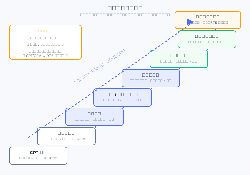
As shown in the figure, this ladder is driven by two forces together: format evolution (content and ads merging, with feed and native formats reducing the harm to experience) and mechanism evolution (from selling slots to selling audiences, CPT/CPM to RTB real-time bidding). The two lines converge at the top at "programmatic trading + nativeness".
Feed Ads: A Positive Example of Balancing Effectiveness and Experience
Along this evolutionary line, Feed Ads / Native Ads deserve special emphasis. A good ad format can balance advertising effectiveness and user experience, and feed ads are a positive example. Their form closely resembles the content users consume, mixed into the reading feed — made possible only by technological progress. Its "balancing" logic shows on both ends: for advertisers, the feed's native form improves attention and acceptance (corresponding to the selection and interpretation phases of the effectiveness model), and exposure is not actively blocked by users; for users, the ad does not interrupt the reading rhythm or cause a jarring experience. This echoes the value formula's warning about the "resource volume" factor — total ad resources are proportional to user usage, and only by protecting user experience can the denominator of usage time keep growing.
💡 Key Insight: The essence of ad format evolution is "ads getting ever closer to content, and trading getting ever closer to the impression". The former solves the user-acceptance problem (the first half of the effectiveness funnel), while the latter solves the pricing-precision problem (the pricing mechanism factor in the value formula). Feed ads happen to stand at the intersection of the two lines — they are both a product of format fusion and the primary carrier of precise targeting and programmatic bidding.
Analysis: Ad formats are relatively mature (banners, video, text links), and are usually not a concern for the advertising system — the first-order factor in ad effectiveness is the design of the ad creative. But "scientific marketing" is changing this: advertising systems are beginning to help advertisers optimize marketing strategy. For algorithm engineers, the more reliable levers remain targeting technology (audience-ad matching) and pricing mechanisms, i.e., this chapter's 12.1.4 and the upcoming 12.2/12.3.
⚠️ Common Mistakes in 12.1
| # | Mistake | Example | Why It's Wrong | Fix |
|---|---|---|---|---|
| 1 | Treating ads as "recommendations with a price" | "Ad ranking is just CTR ranking plus a bid" | Advertising involves a three-party game of interests (users/advertisers/media), and bids make matching non-homogeneous | Use the eCPM lens to unify click-through rate and click value, balancing all three parties |
| 2 | Believing "more precise is more valuable" or "precision + big data necessarily boosts revenue" | Blindly pursuing targeting with an extremely narrow audience | Data sources with low audience coverage are also valuable; there is a trade-off between reach and precision | Evaluate targeting value by looking at both reach and quality |
| 3 | Confusing Ad Networks with the ADX | "An Ad Network is just a small Ad Exchange" | Ad networks are closed systems that sell audiences with CPC pricing; the ADX is open real-time auctioning, bidding per impression | Remember the boundary: 2.0 closed networks vs. 3.0 open trading |
| 4 | Ignoring Cookie Mapping's foundational status | "The DSP can identify the user as soon as it receives a bid request" | The ADX's bid request carries the media Cookie; the DSP must first look up the mapping table to map it to its own user ID | Understand Cookie Mapping as step 0 of RTB |
| 5 | Thinking RTB is only the multi-bidder auction step | "RTB is just the ADX collecting bids and taking the highest" | RTB includes two phases, Cookie Mapping and Ad Call, plus two costs: latency (a ~100ms budget) and privacy | Use the seven-step sequence diagram to understand the full chain |
| 6 | Equating personalized retargeting with "winning back old customers" | "Retargeting is just re-serving ads to people who visited" | Personalized retargeting must push item-granularity ads, remove already-purchased items, and recommend related new arrivals — essentially an offsite recommendation engine | View it as a reuse of the recommender system's ranking technology on ad slots |
Chapter Summary
📌 Key Takeaways
| Concept | Key Points | Why It Matters |
|---|---|---|
| Definition of advertising | The three elements — sponsor / medium / audience; essence is low-cost user contact | The cost advantage of "non-personal" communication is the foundation of the advertising business model |
| Effectiveness model | Exposure→Attention→Comprehension→Acceptance→Retention→Decision, grouped into three phases | The framework for ad effectiveness evaluation and format design; parallels the recommendation funnel but finer |
| Fundamental problem | matching to maximize ROI | Context is a first-class citizen, and matching is non-homogeneous due to bids |
| Differences from recommendation | Homogeneous vs. non-homogeneous, endpoint vs. downstream, interest diversity vs. return rate | The cognitive anchorpoint for engineers moving from recommendation to advertising |
| Value formula | Conversion efficiency × pricing mechanism × resource volume × delivery efficiency | The master framework for understanding advertising technology evolution |
| Delivery models 1.0–3.0 | Direct contracts → Ad Networks (sell audiences, CPC) → programmatic trading (DSP-ADX-SSP-DMP) | Each generation solves the previous one's problems while introducing new costs (closedness/latency/privacy) |
| RTB | Two phases — Cookie Mapping + Ad Call; seven-step sequence; ~100ms budget | The core mechanism and engineering constraints of programmatic trading |
| Trading method spectrum | Premium Sale (guaranteed delivery) → Preferred Deal → Network Optimization → RTB | Different traffic matches different transaction granularity; the SSP's yield optimization does the routing |
| Three stages of targeting | Rule-based → data-based → system-based (Retargeting/Look-alike) | Personalized retargeting = offsite recommendation engine, directly sharing roots with recommendation technology |
| Feed ads | Content and ads fused; a positive example of balancing effectiveness and user experience | The convergence point of format evolution and mechanism evolution |
❓ FAQ
Q1: Who bears the risk of click-through rate estimation in CPC and CPA markets, respectively?
A: In the CPC market, click value is declared by the advertiser through bidding, while the click-through rate is dynamically estimated by the platform — the risk lies mainly in the platform's estimation ability; in the CPA/CPS market, both the click-through rate and click value are dynamic, all decisions rest with the platform, and the conversion risk falls entirely on the platform — which is why only markets whose advertisers have highly uniform conversion processes (e.g., Taobao) are suitable for building on CPA/CPS.
Q2: Why can't Ad Networks easily support customized audience segmentation, while DSPs can?
A: The Ad Network is a closed system, where advertisers can only "clearly describe" their needs using the network's preset tags; the DSP has customized audience segmentation capabilities, can connect advertiser data (seed audiences, Cookie embedding), and bid on network-wide traffic by the advertiser's own audience definition — this is exactly the core driving force of the move from 2.0 to 3.0.
Q3: What is the relationship of search retargeting to personalized retargeting and look-alike, respectively?
A: Personalized retargeting is the vertical extension of retargeting, doing item-granularity personalized delivery to already-reached users (an offsite recommendation engine); search retargeting is the horizontal extension, directing users who have searched related keywords to the advertiser's site — strictly speaking it targets unreached users, so its nature is closer to look-alike.
🔗 Connections to Later Chapters
- 12.2 (CTR estimation) expands on the "dynamic click-through rate estimation" that recurs throughout this chapter — ad ranking needs accurate absolute CTR values, not merely a relative ordering, which is exactly the value of the regression task.
- 12.3 (auctions and mechanism design) picks up the trading method spectrum: GSP/VCG pricing, position auctions, and the mechanism details of eCPM ranking.
- 2.x (retrieval) — ItemCF / vector retrieval is isomorphic to this chapter's targeting technology: retargeting and look-alike are essentially "retrieval with an audience as the query".
- 3.x (ranking models) — CTR models (e.g., DeepFM, DIN) directly serve advertising's eCPM ranking; for industrial practice, see Alimama's DIN / DIEN and Meituan's search ad ranking in the further reading.
- 8.3 (end-to-end generative advertising) shows the frontier form of unifying auction mechanisms with generative models, which can be viewed as this chapter's programmatic ecosystem projected onto the model layer.
Practice Problems
Work through all problems in order — they get progressively harder. Each has a complete solution you can reveal after trying it yourself.
Problem 12.1.1 — Advertising Definition and Classification 🟢 Easy
Judge whether each of the following 4 statements is true or false, with a one-sentence justification each: (a) "Non-personal" in the advertising definition means ads do not need a sponsor; (b) the typical metric of brand advertising is short-term conversion rate; (c) "Attention" in the effectiveness model belongs to the selection phase; (d) display ads have a low click-through rate and should therefore be abandoned.
💡 Solution (click to reveal)
Approach: Check each statement against the definition and model in 12.1.0.
- (a) False. The three elements of advertising are sponsor, medium, and audience; "non-personal" emphasizes not relying on face-to-face personal selling and achieving low-cost user contact — the sponsor remains an essential element.
- (b) False. Brand Awareness advertising focuses on long-term influence and building recognition; pursuing short-term conversion actions is the hallmark of Direct Response advertising.
- (c) True. The selection phase contains Exposure and Attention (being seen); the interpretation phase contains Comprehension and Acceptance; the attitude phase contains Retention and Decision.
- (d) False. Although the display-ad end of the online advertising channel spectrum has low conversion rates, it attracts more potential customers and raises the conversion rates of downstream channels (SEM, paid product listing, etc.) — an impression is itself a valuable user contact.
Key points:
- None of the three elements can be omitted; "non-personal" is the source of the cost advantage.
- Funnel evaluation must look at the synergy of the whole chain, not just single-point metrics.
Problem 12.1.2 — Risk Allocation in CPM/CPC/CPA 🟢 Easy
An ad platform is deciding which pricing market to adopt. Advertisers want to "pay only for final sales"; the platform is confident in its CTR estimation ability but unsure about the differences in conversion processes across advertisers. Answer: (a) In a CPA/CPS market, who makes the decisions on click-through rate and click value, respectively? (b) Why could Taobao's advertising platform adopt CPA/CPS as its foundation? (c) Which market should the platform choose in this case?
💡 Solution (click to reveal)
Approach: Use "who dynamically decides which term" to analyze risk attribution.
- (a) In a CPA/CPS market, both the click-through rate and click value are dynamic, equivalent to the platform making all decisions, with the risk falling on the platform.
- (b) Taobao's advertisers (sellers) follow roughly the same service process, so the platform has a consistent grasp of different advertisers' conversion chains, keeping the risk controllable.
- (c) The platform is confident in CTR estimation but unsure about advertiser conversion differences; the CPC market is exactly "click value judged by the advertiser (bidding), click-through rate dynamically estimated by the platform" — each side dynamically decides the term it knows best, so choose CPC.
Key points:
- CPM: decisions and risk all on the advertiser; CPC: each side handles one; CPA/CPS: decisions and risk all on the platform.
- The choice of pricing mechanism is essentially a match between risk and informational advantage.
Problem 12.1.3 — The RTB Chain and Its Latency Cost 🟡 Medium
Arrange the 7 steps of one RTB impression in the order they occur (using numbers ①–⑦): ① the DSP estimates eCPM and bids; ② the user visits a media page, triggering an ad request; ③ the ADX broadcasts the bid request to each DSP; ④ the SSP wraps the traffic information and initiates the ad request; ⑤ auction settlement — the highest bidder wins the impression; ⑥ the winning ad is returned; ⑦ the ad is rendered and shown to the user. Also answer: why is RTB said to carry "two costs"?
💡 Solution (click to reveal)
Approach: Check against the RTB sequence diagram (the Ad Call phase).
Correct order: ② → ④ → ③ → ① → ⑤ → ⑥ → ⑦.
The two costs:
- Latency: compared with returning an ad directly, RTB adds one Round Trip (the bid-request/bid round trip between the ADX and DSPs); the entire chain must be kept within a budget of roughly 100ms, otherwise the user perceives a blank screen.
- Privacy: the bid request carries user identifiers and page information broadcast to multiple DSPs, creating a risk of browsing-data leakage.
Also, don't forget the precondition: all of this rests on Cookie Mapping (initiated by the DSP, loading an iframe on the demand-side website, with the mapping table stored on the Demand side) — without the identity lookup, the DSP cannot identify the user even when it receives a bid request.
Key points:
- Cookie Mapping is step 0; the Ad Call is the bidding flow for every impression.
- Transaction granularity (single impression) versus communication cost is RTB's inherent trade-off.
Problem 12.1.4 — Choosing a Targeting Solution 🔴 Hard
A cross-border e-commerce company hires you as a delivery consultant. Its three requirements and the available targeting technologies are below; pick the most suitable technology for each and justify the choice: (a) "Users who added items to cart last month but didn't order — I want to separately push the items in their carts and similar new arrivals"; (b) "We have a list of 50,000 high-value existing customers, and want to find more people like them"; (c) "Limited budget — I only want to target people who recently searched 'overseas baby formula' on search engines".
💡 Solution (click to reveal)
Approach: Match the technology by targeting object (already-reached users / seed expansion / search behavior).
- (a) Personalized retargeting (the vertical extension of retargeting). The targets are users already reached on the advertiser's own site (identified via Cookie embedding); push item-granularity ads: cart-item reminders, removing already-purchased items, recommending similar new arrivals — essentially putting the on-site recommendation showcase into media ad slots (an offsite recommendation engine).
- (b) Look-alike. Take the 50,000 existing customers as the seed audience; the DSP finds potential new users among the supply-side audience by behavioral similarity; at the same reach level, it performs better than generic tag targeting. Note: use non-Demand-side data as much as possible to avoid reselling users between competitors; also, "similar" is a black box, so effectiveness needs experimental validation.
- (c) Search retargeting. Analyze the advertiser's traffic originating from search engines, and direct users who searched specific keywords to the advertiser's site; strictly speaking it targets unreached users, so its nature is closer to look-alike — but with search terms as the signal, intent strength is high and budget efficiency is good.
Key points:
- The first question in choosing a targeting technology: is the target audience "already reached" or "not yet reached"?
- Behavior strength spectrum: the closer to demand and the more active a behavior, the greater its contribution to conversion — search clicks beat ad clicks, which beat page views.
🏆 Challenge: Planning a Trading Method Mix for a New Ad Product
You are in charge of ad monetization for a news app with tens of millions of daily active users. The product has three ad slot types — homepage splash, in-feed mixed placement, and article bottom — and the advertiser mix is 60% brand advertisers + 40% performance advertisers. Write about 180 words explaining how you would assign trading methods across the "Premium Sale (guaranteed delivery) / Preferred Deal / Network Optimization / RTB" spectrum for the three slot types, and what to watch in the feed slot's format design.
💡 Hint
A reference allocation: the splash slot has high exposure volume and strong exclusivity, suiting brand advertisers for Premium Sale (guaranteed delivery, CPT/CPM settlement, volume over quality, requiring traffic forecasting and online allocation to fulfill the contracted volume); the feed has the largest traffic but dispersed per-impression value, suiting connection to RTB open auction for full price discovery (while reserving Preferred Deal for top advertisers with strong bargaining power to pick premium traffic first); the article-bottom long-tail traffic has low unit value — just connect it to an Ad Network for network optimization, saving RTB's communication cost. In format, the feed should make ads resemble the content forms users consume (image-and-text cards mixed in) without interrupting the reading rhythm — feed ads are exactly "a positive example of balancing ad effectiveness and user experience"; protecting user experience protects the long-term denominator of "usage time → resource volume". Core logic: different ad slots have different traffic characteristics, and the SSP's yield optimization should pick the highest-eCPM monetization channel on the spectrum for each piece of traffic.
Billing Models and Core Metrics
📝 Before You Continue: Please read 12.1 (the advertising ecosystem panorama) first, to understand the division of roles among advertisers, media, and platforms along the transaction chain. The CTR modeling in 12.2.4 of this chapter carries the same lineage as the ranking models of Part 3 — if you have already read the CTR models in 3.x, you can treat this chapter as their "economic restatement" in the advertising setting.
You type "running shoes" into a search box, and the first result on the page is an ad — why does it deserve that spot? How much does the platform expect to earn from that single impression? Behind these questions lies no mystical algorithmic black box; the answer is written in two things: the Billing Model, which determines who pays at which step, and Metrics, which determine the yardstick the system uses to compare candidate ads.
Recommender systems optimize a fuzzy blend of user experience and business goals, whereas advertising systems have had "money" written into their objective function from day one. The billing model acts as a constitution: it stipulates how risk is allocated between advertisers and media, and every downstream component — retrieval, ranking, traffic forecasting, exploration strategies — must operate within its frame. Change the billing model, and the shape of the entire tech stack changes with it.
This chapter starts from the clash between the value models of advertisers and media, walks the billing spectrum from CPT to CPS, builds the ranking logic with eCPM as the unified measure, and then dives into the engineering details of guaranteed-contract online allocation and click-through rate estimation. All of this is the foundation for the auction mechanisms of 12.3 — you must first understand "how the bill is computed" before you can understand "how the price is set".
After reading this chapter, you will be able to:
- List the billing formulas, key decision-makers, and risk allocation of each billing model: CPT/CPD, CPM, CPC, and CPA/CPS
- Characterize ad performance with the three metrics CTR, CVR, and ROI, and carry out cross-billing-model ranking computations with
- Explain the divide between brand advertising and direct response advertising in billing and transaction modes
- Describe the bipartite-graph structure of Guaranteed Delivery (GD) and Online Allocation, and the ideas behind solving them
- Explain why CTR estimation is a regression problem rather than a ranking problem, along with cold-start back-off and E&E as coping strategies
- Complete 5 graded practice problems, working through the computational chain from metric conversion to GSP payments
12.2.0 Why the Billing Model Is the "Constitution" of an Advertising System
Every commercial product must answer the question "how do we collect money", but what makes online advertising special is this: the choice of billing unit is, in essence, an allocation of the risk created by outcome uncertainty. From impression to click to conversion, each step forward carries more uncertainty; charging at a given step amounts to pushing all risk downstream of that step onto one party. That is why the billing model is the constitution of an advertising system — it precedes every algorithm and defines the rules of the game.
Start from the Advertiser's side. The core of the advertiser's value model is to derive the value of a single ad backward from its final outcome. Suppose the marketing cost of selling one car is 2,000 yuan and the conversion rate from ad impression to completed purchase is 0.1%; then the value of one ad impression is yuan — no matter how golden the media considers its homepage banner, the scale in the advertiser's mind recognizes only this number. Real-world computations are more involved, but the principle stands: work backward from the money. By this logic, Cost Per Action (CPA) or even Cost Per Sales (CPS) pricing is the closest fit to the advertiser's value model.
Now stand on the side of the media / Supply Side. What the media cares about is not how many cars the advertiser can sell, but how much revenue each unit of ad inventory can generate — what the homepage banner is worth today, and whether it will still be worth that tomorrow. This naturally gives rise to "sell-the-resource" pricing models such as Cost Per Time (CPT) and Cost Per Mille (CPM): treat the ad slot as a shop front awaiting tenants, with direct measurement and stable income.
Clearly, the two sides perceive "ad inventory usage" differently, so a game is inevitable — one misconception to guard against is that media interests and advertiser interests are locked in a correlated game, not aligned. The eventual outcome of this game is that ad measurement evolved into two major categories. Direct Response advertising: the supply side computes ad volume from ad performance; this model originally served advertiser interests — early on it could indeed hurt the supply side, because when ad creatives were poor, click-through rates stayed low even with heavy exposure allocation. As technology advanced, however, this problem was overcome: by analyzing data such as ad click-through rates, the system automatically lowers the delivery share of these "low-profit" ads or demands higher bids from advertisers. Brand Awareness advertising: billed by impressions, which is more straightforward for the supply side and better suited to ad demand with no direct conversion goal (such as new-product awareness).
🧠 Mental Model: Three Ways to Collect Rent from a Shop Front
Think of the media as a landlord. CPT is "leasing the whole building": the tenant pays fixed rent; whether business thrives or dies is no business of the landlord's, and all risk sits with the tenant. CPC is "charging per store visitor": the landlord must attract foot traffic likely to walk in, while the tenant pays for every person who enters. CPS is the "pure-commission clerk": a cut only when something sells, nothing when it doesn't — all risk falls on the platform doing the hawking. Every move along the billing-model spectrum is, in essence, a redistribution of risk between landlord and tenant.
Analysis: The choice of billing model is not a purely technical decision; it depends on both parties' data capabilities and their control over the conversion funnel. CPA/CPS-style settlement only becomes truly viable when the platform has sufficient control over the full "impression-to-purchase" funnel and the advertisers (sellers) share roughly the same service workflow — Taobao's advertising platform, for example. The less controllable the funnel, the more the billing unit must shrink back toward the impression end.
12.2.1 The Billing Spectrum: From Buying Time to Buying Sales
With "risk allocation" as the key, we can arrange the mainstream billing models along a spectrum: from buying out time, to paying per impression, per click, per action, per sale. The closer the billing unit sits to the final conversion, the better it fits the advertiser's value model — and the more risk the platform takes on.
Cost Per Time (CPT) and Cost Per Day (CPD) sit at the far left of the spectrum. Many websites in China still sell ad slots on a fixed "X yuan per month" basis; Alimama's weekly-billed ads and portal sites' monthly banner deals belong to this category. It is crude — who saw the impression, whether anyone looked at all, is unknown, so the client's interests cannot be guaranteed — but it is also hassle-free and brings the website stable income, which is why it is common in contracted brand advertising, occupying the core banner modules of major websites. Compared with CPS, CPD places modest demands on the foundations of a partnership and makes deals easy to strike; its weakness is that, over long-term cooperation, it is less real-time and effective than CPS.
Cost Per Mille (CPM) takes the first step toward performance:
where "Spend" is what the advertiser pays to run the ad. CPM means cost per thousand impressions: charging by exposure volume started advertising's evolution toward "performance orientation", and it is also a common billing method in RTB (Real-Time Bidding) systems. Cost Per Click (CPC) goes one step further:
Keyword advertising and other performance-based formats generally adopt this pricing model; it is likewise the mainstream billing method in RTB. Cost Per Action (CPA) charges according to the actions each visitor takes on the ad, where "action" has a specific definition — completing a transaction, acquiring a registered user, and so on. Cost Per Sales (CPS) converts the ad placement fee into a commission on actual product sales: to hedge against ad-spend risk, the advertiser pays a commission on the actual sales generated after the click, commonly seen in the billing of small websites inside affiliate networks.
dCPM (dynamic CPM) deserves a separate word. It is the settlement system widely adopted by DSPs (Demand-Side Platforms): unlike the fixed CPM spoken of in the market (called flat CPM accordingly), dCPM was born on RTB technology and means that the bid for every single impression varies. Each bid is computed in real time from the performance of the advertiser's campaign (usually CPS), yielding the price most favorable to the advertiser and thus protecting the advertiser's interests; and because settlement with the media is still per impression, the media's revenue is also secured. In one sentence: settle with the media by impressions, optimize for the advertiser by performance — dCPM is precisely an engineering resolution of the two-sided game we described in 12.2.0.
As shown, the left end of the spectrum presses risk onto the advertiser's shoulders, the right end onto the platform's, with CPC balancing in between. More precisely, risk allocation can be labeled by "who makes the key decision": in a CPM market the eCPM is fixed, which amounts to handing all decisions (and risk) to the advertiser — the platform guarantees impressions, but whether they bring clicks and conversions afterwards is none of its business. The CPC market is the compromise: the value of a click is judged by the advertiser (expressed in the bid), while the click-through rate is dynamically estimated by the platform, which knows the traffic better (Google, for example) — the platform uses CTR prediction to manage the share of risk it carries. In CPA/CPS markets both are dynamic, which amounts to the platform making the decisions and bearing the risk; Taobao's advertising platform adopts this kind of settlement precisely because its advertisers (sellers) share roughly identical service workflows and the platform's grip on the conversion funnel is strong enough.
| Billing Model | Billing Unit | Who Makes the Key Decision | Risk Allocation | Typical Scenarios |
|---|---|---|---|---|
| CPT/CPD | Time slot / day | Media sets price, advertiser buys out | Advertiser | Brand takeovers, core banners |
| CPM | Per thousand impressions | Platform guarantees volume, eCPM fixed | Advertiser | RTB display bidding, GD contracts |
| CPC | Per click | Advertiser sets click value, platform estimates CTR | Shared by both (compromise) | Keyword ads, ad networks |
| CPA | Per action | Platform | Platform | Ecosystems with standardized service workflows (e.g., Taobao) |
| CPS | Per sale | Platform | Platform | Affiliate networks, rebate sites |
💡 Key Insight: Economics has a saying, "price fluctuates around value", and a good pricing mechanism should let price approach value as closely as possible. But advertisers and supply sides are naturally misaligned in how they perceive "value", so static pricing never closes the deal — and the market's answer is to let the market price itself. Auctioning is the pricing method both sides can currently accept; its core questions are how to get more demand-side participants into the auction and how to offer finer-grained bidding — exactly the subject of 12.3.
12.2.2 The Core Metric System: eCPM as the Unified Measure
The billing model sets the rules; a set of metrics is still needed to measure "how well the rules are being executed". Three foundational performance metrics form the common language of advertising data analysis.
Click-Through Rate (CTR) measures the average number of user clicks an ad receives across multiple impressions:
Conversion Rate (CVR) measures the relationship between user clicks and final orders:
Return On Investment (ROI) measures the relationship between the order value generated by the advertiser's ad spend and the spend itself:
These three metrics stack on one another: CTR is the platform's "supply-side metric" — it determines traffic quality; CVR connects clicks to conversions, characterizing the quality of demand; and ROI is what the advertiser ultimately votes with — advertisers whose ROI stays below 1 (or the industry-acceptable threshold) vote with their feet and pull their budgets.
Here is the problem: when a CPC-billed ad and a CPM-billed ad compete in the same auction, how does the platform compare them? The answer is eCPM (effective CPM) — the expected revenue per thousand impressions, which converts every billing model onto the same ruler:
- Under CPC billing: . Here pCTR is the platform's estimate of the click-through rate for this impression, and bid is the advertiser's per-click price; multiplying the two gives the "expected revenue per impression", and multiplying by 1000 converts it to a per-thousand-impression basis.
- Under CPM billing: . A thousand impressions cost exactly that much, so the expected revenue is the bid itself.
The platform's ranking logic then falls out naturally: for each impression opportunity, convert all candidate ads to eCPM and sort them in descending eCPM order, allocating slots in turn. Consider a numerical example: Ad A bids 2.0 yuan with pCTR 3%, Ad B bids 5.0 yuan with pCTR 1%, and Ad C bids 1.0 yuan with pCTR 8%. Their eCPMs are yuan, yuan, and yuan respectively. B, the highest bidder, lands at the bottom — its click probability is too low, so winning this impression would not pay off for the platform; C wins in the end.
As shown, eCPM is the "common currency" of the ad market: wherever a candidate comes from, it must first be exchanged into eCPM before it can compete on the same stage. This also explains why 12.2.0 called the billing model a constitution — the shape of the eCPM formula is entirely determined by the billing model, and whether pCTR is accurate (12.2.4) directly determines whether this ruler measures true.
🧠 Mental Model: The Airport Currency Exchange
Imagine a duty-free shop that accepts dollars, euros, and yen at once. The cashier does not compare the three currencies directly; everything is first converted into dollars at the exchange rate before being priced. eCPM is the exchange counter of ad trading: CPC's "dollars", CPM's "euros", and CPA's "yen" are all converted into "expected revenue per thousand impressions". Get the exchange rate (pCTR, bid) wrong and the price tag is distorted — which is exactly the weight the next section's CTR estimation carries.
Finally, the two advertising forms from 12.2.0 converge here: brand advertising is billed by impressions and traded through contracts (CPT/CPD/CPM, focused on long-term impact), while direct response advertising is billed by outcomes and traded through auctions (CPC/CPA/CPS, chasing short-term conversion actions). The two diverge in delivery timing, creative formats, and system modules — but once they enter the same ad slot, the platform still rules on both with the same eCPM ruler.
12.2.3 Guaranteed Contracts and Online Allocation: Volume First, Quality Second
Auctions are the star of modern advertising, but before them, guaranteed contracts ruled the first decade of Internet advertising and still hold the high-end brand budgets today. Understanding them is a necessary step toward understanding the evolution of the whole advertising system.
Guaranteed Delivery (GD) is the core mechanism of contract advertising. Its essentials can be summarized as: a contract-based ad mechanism where the agreed impression volume must be compensated if unmet; a "volume before quality" approach — secure the volume first, optimize later; CPM settlement; and delivery decided server-side (rather than in real time at auction). GD's audience targeting rests on two prediction technologies: click-through rate prediction and traffic forecasting — the former estimates "how an impression performs on a given audience", the latter estimates "how much of a given type of traffic the future holds"; together they underwrite the promise of "whether the contracted volume can be fulfilled within the term".
The technical core of contract advertising is the Online Allocation problem: modeling the matching of ads to traffic as a bipartite-graph optimization of Ad → (Context, User). One side of the graph holds ad contracts carrying targeting conditions; the other holds the stream of traffic supply jointly characterized by (context, user); each time an impression arrives, the system must complete the allocation under the constraint of "fulfilling every advertiser's contracted volume". The objective function can be adjusted as needed (say, maximizing total revenue or total clicks), and the classic solution is to construct and solve the dual problem — turning each contract's volume constraint into a dual variable (a shadow price), so that online allocation decisions are made on the net gain of "revenue minus shadow price".
As shown, contract ① (an automotive brand, targeting males 25–40) can match traffic from (sports channel, male users), and can also filter its target audience out of (homepage feed, all users); contract ③ has no targeting restriction, so it connects to every supply node. On top of the supply volumes given by traffic forecasting, the allocation algorithm must pick for each piece of traffic a contract that "both fulfills the volume guarantee and maximizes value".
Traffic forecasting is itself an interesting problem: it can be viewed as an inverted retrieval problem, where the ad is the query and the space is what gets retrieved. The difficulty lies in the sheer size of the joint space, which forces and to be handled separately — the exact flip side of the forward direction, "retrieving ads with user requests".
Analysis: The division of labor between online allocation and auctions (12.3) can be understood as follows: contracts sell coarse targeting granularity (by audience packages and channels), auctions sell fine granularity (down to a single impression, a single bid); contracts sell certainty (guaranteed volume, compensation), auctions sell uncertainty (highest bidder wins). GD's weaknesses are that its audience targeting categories lack fine detail, and in contract sales brand advertisers impose exclusivity requirements on exposure (e.g., competitor exclusion), which further tightens the freedom of allocation. When both traffic supply and demand in a market are dense enough, coarse-grained contracts gradually give way to fine-grained auctions — this is the economic driver behind advertising's shift from impression-volume contracts to RTB.
12.2.4 Click-Through Rate Prediction: Ranking Models Take On a New Mission
12.2.2 planted the seed: under CPC billing, eCPM = pCTR × bid × 1000, so the accuracy of CTR estimation directly determines whether the ranking ruler measures true. Now we treat CTR estimation as a standalone modeling problem — it shares its origins with the ranking models you met in Part 3, yet meets a different fate.
The standard form of CTR prediction is the probability model : given ad , user , and context , estimate the probability that the user clicks. You might think: isn't this just the Part 3 CTR model in a new setting? The model architecture can indeed be reused, but the nature of the task changes — regression fits better than ranking. A recommender's ranking model only needs the relative order among candidates to be correct (a high AUC suffices), while the actual ranking basis in advertising is eCPM: the CTR estimate gets multiplied by the bid before comparison. A model that systematically overestimates CTR pushes low-bid ads up to positions they don't deserve; systematic underestimation does the opposite. In other words, an advertising system needs CTR absolute values that are as accurate as possible, not merely correct relative ordering among candidates — this is the first principle distinguishing CTR modeling from recommendation ranking.
New-Ad Cold Start: Hierarchical Back-off
A newly launched ad has no click statistics, so where does its pCTR come from? The answer is to exploit the ad hierarchy: creative → solution → campaign → advertiser. A new creative has no statistics, but its campaign might; if the campaign doesn't either, back off one more level to the advertiser, estimating from the historical CTRs and ad labels of the same advertiser's past ads. This back-off strategy mirrors how recommender systems handle new items: structural priors make up for missing statistics.
Dynamic Nature: The Trade-off Between Dynamic Features and Online Learning
The distribution of the ad market shifts extremely fast — creative fatigue, seasonal swings, and breaking topics can render yesterday's trained model inaccurate today. There are two directions of response, each with its cost. Dynamic features: aggregate click-feedback statistics along label-combination dimensions and feed them to the model as features (i.e., multi-level click feedback); the hallmark is "fast-adjusting features" — the model stays fixed while the features change in real time. Its advantages are a scalable engineering architecture and strong back-off for new combinations; its drawbacks are heavy online feature storage and demanding update requirements. Online learning: let the model itself update in a streaming fashion on new data, "fast-adjusting the model", at the cost of engineering complexity in training and serving. Industrial systems often use both: dynamic features absorb short-period fluctuations, while online learning keeps pace with medium-to-long-term drift.
Exploration and Exploitation: Accumulating Statistics for Long-Tail Combinations
However good the features and however new the model, one cold fact remains: the combination space is nearly infinite, the vast majority of combinations have never received an impression, and their CTR is beyond estimation. The task of the Exploration & Exploitation (E&E) framework is exactly this: create suitable impression opportunities for long-tail combinations to accumulate statistics, thereby estimating CTR more accurately and lifting overall ad revenue. Exploration is not charity — today's "waste" is an investment in tomorrow's more accurate estimates; but both the volume and the effectiveness of exploration must be strictly controlled, or it directly erodes current revenue. Three classic strategies:
- ε-greedy: explore randomly on an ε fraction of traffic, exploit the current best on the rest. The simplest to implement, and the least exploration-efficient.
- UCB (Upper Confidence Bound): compute an upper confidence bound on the expected reward for every candidate and pick the arm with the highest UCB; the more often an arm is selected, the closer its UCB gets to the true expected reward — naturally balancing "try more of the untried" with "use more of the well-performing".
- Contextual Bandit: for each impression, make decisions on the arm's feature vector instead of the arm itself, achieving dimensionality reduction — no need to estimate separately for every specific ad; generalize in feature space instead, neatly echoing the hierarchical idea of back-off.
Analysis: The suitability of the three E&E strategies in advertising: ε-greedy works as a fallback strategy or in the early cold-start stage; UCB pays off clearly when the candidate set is small, but with huge candidate counts both the bound computation and the storage become burdens; Contextual Bandit sidesteps candidate explosion through feature-based dimensionality reduction and is the mainstream form of exploration modules in modern ad systems. The shared principle: exploration traffic must be spent where it counts — prioritize the long-tail combinations whose accurate estimation would lift expected revenue the most.
At this point, the decision chain of an ad request is complete: candidate ads enter ranking through targeted retrieval, the pCTR model outputs click probabilities, they are multiplied by bids and converted into eCPM, sorted descending, and impressions allocated from the top down. But note — eCPM ranking is only the entry ticket: it decides who takes the stage; what actually decides "how much the platform collects" is the auction mechanism. The same eCPM winner, paying under the GSP (Generalized Second Price) mechanism, may pay a price far from its own bid. Who should pay how much, why truthful bidding may (or may not) be the optimal strategy, and how VCG prices via "externalities" — these questions belong to the territory of mechanism design, which we unfold in 12.3.
⚠️ Common Mistakes in 12.2
| # | Mistake | Example | Why It's Wrong | Fix |
|---|---|---|---|---|
| 1 | Treating CTR estimation as a ranking problem | "A high AUC is all that matters; absolute values don't" | Ads rank by eCPM, where CTR gets multiplied by the bid; systematic over/underestimation changes both ranking and billing | Evaluate it as a regression/calibration problem; watch the deviation between predicted and true absolute values |
| 2 | Confusing eCPM with CPM | "eCPM is just cost per thousand impressions" | CPM is a billing model (a cost measure); eCPM is the expected revenue per thousand impressions (a revenue measure) and the unified measure for ranking | Remember e = expected/effective; eCPM serves the platform's ranking decisions |
| 3 | Assuming CPA/CPS is better for the platform | "Performance-based billing must mean the platform earns more" | Under CPA/CPS both CTR and value are dynamic; decisions and risk fall entirely on the platform, which bleeds money when the conversion funnel is uncontrollable | It only suits ecosystems with strong funnel control and standardized service workflows (e.g., Taobao) |
| 4 | Assuming more precise targeting always creates more market value | "Precise targeting + big data will surely boost revenue significantly" | Media and advertisers are in a correlated game; who captures the gains of precision depends on the billing and pricing mechanisms | Analyze each party's incentives from the angles of risk allocation and game theory |
| 5 | Ignoring the difference between dCPM and flat CPM | "Isn't dCPM just CPM?" | flat CPM fixes the per-thousand price; dCPM's bid for every impression changes in real time with campaign performance | Distinguish the two ledgers: "settling with media by impressions" vs. "optimizing for advertisers by performance" |
| 6 | Doing contract allocation with CTR prediction but no traffic forecasting | "An accurate model is enough to fulfill the volume guarantee" | GD's volume constraints rest on traffic forecasting; misestimate the supply and the guarantee inevitably collapses | Online allocation = CTR prediction + traffic forecasting; neither can be missing |
Chapter Summary
📌 Key Takeaways
| Concept | Key Points | Why It Matters |
|---|---|---|
| Billing model as constitution | The billing unit determines risk allocation: advertisers derive value backward from outcomes, media care about revenue per unit of inventory | Every ad algorithm operates under the rules of the game drawn by the billing model |
| The billing spectrum | CPT/CPD → CPM → CPC → CPA/CPS, risk shifting gradually from advertiser to platform | A platform that picks the wrong billing model takes the risk onto itself |
| Three core metrics | CTR = clicks/impressions, CVR = orders/clicks, ROI = order value/spend | The common language of advertising data analysis |
| eCPM | Under CPC = pCTR×bid×1000; under CPM = bid; rank descending by it | The unified measure across billing models, the ruler of ranking |
| GD and online allocation | Guaranteed volume with compensation for shortfall, volume before quality, CPM settlement; Ad→(Context,User) bipartite graph solved via duality | The technical core of contract advertising, the coarse-grained counterpart to fine-grained auctions |
| CTR estimation | Regression, not ranking (absolute accuracy required); cold start via creative→advertiser hierarchical back-off; dynamic features vs. online learning; E&E to accumulate long-tail statistics | The accuracy of eCPM ranking depends entirely on pCTR calibration |
❓ FAQ
Q1: Under CPC billing, how does the platform manage the risk it bears?
A: The platform knows click-through rates better (Google, for example) and manages the uncertainty of "will this impression be clicked" through CTR estimation: lowering the delivery share of low-pCTR ads or demanding higher bids. This is exactly why CPC is called the compromise point of risk — the advertiser judges the click's value and bids, while the platform estimates the CTR and shoulders traffic quality.
Q2: Why does eCPM equal the bid under CPM billing?
A: CPM billing charges per thousand impressions, so the advertiser's bid is itself "what I'm willing to pay per thousand impressions" — that is, the platform's expected revenue per thousand impressions, with no need to multiply by pCTR. It also means the eCPM in a CPM market is fixed, handing all decisions and risk to the advertiser.
Q3: What is the essential difference between contract ads and auction ads?
A: Three points. Transaction mode: contracts are negotiated-ahead guaranteed sales, auctions are real-time trades. Billing: contracts settle on CPM impression volume, volume before quality; auctions bill by performance such as CPC/CPA. Targeting granularity: contracts sell coarse-grained audience packages/channels with brand exclusivity demands, while auctions can go as fine as a single impression. The denser the market's supply and demand, the more it favors fine-grained auctions.
🔗 Connections to Later Chapters
- The division of roles among advertisers, media, and platform in 12.1 (the advertising ecosystem panorama) is the premise of this chapter's risk-allocation analysis.
- 12.3 (auction mechanisms) picks up where this chapter ends: eCPM ranking decides who takes the stage, while GSP/VCG and other mechanisms decide how much is collected.
- The CTR model architectures of 3.x (ranking models) are the basis of this chapter's pCTR modeling, but the advertising setting raises the bar for absolute-value calibration.
- 8.3 (end-to-end generative advertising) embeds the auction mechanism inside generative models, which can be seen as the unification of this chapter's eCPM ranking and 12.3's auction mechanisms under a frontier architecture.
Practice Problems
Work through all problems in order — they get progressively harder. Each has a complete solution you can reveal after trying it yourself.
Problem 12.2.1 — Metric Conversion 🟢 Easy
An e-commerce advertiser spends 600 yuan in one day, gaining 150,000 impressions, 3,000 clicks, and 120 orders totaling 3,600 yuan. Compute CPM, CPC, CTR, CVR, and ROI.
Sample Input: spend 600 yuan; impressions 150,000; clicks 3,000; orders 120; order value 3,600 yuan
Sample Output: CPM = 4 yuan, CPC = 0.2 yuan, CTR = 2%, CVR = 4%, ROI = 6
💡 Solution (click to reveal)
Approach: Apply the formulas of the five metrics directly.
Key points:
- CPM and CPC convert into each other via ; plugging in verifies the consistency.
- ROI = 6 means every 1 yuan of ad spend brings 6 yuan of order value — the core basis on which advertisers renew their budgets.
Problem 12.2.2 — eCPM Ranking 🟡 Medium
A single request to an ad slot receives three CPC-billed candidates: Ad A bids 1.5 yuan with pCTR 2%; Ad B bids 6.0 yuan with pCTR 0.5%; Ad C bids 3.0 yuan with pCTR 1.2%. Compute each eCPM and give the display order. If a CPM-billed Ad D also bids 40 yuan directly (per thousand impressions), where should it rank?
💡 Solution (click to reveal)
Approach: Under CPC billing use ; under CPM billing the eCPM is the bid itself.
- A: yuan
- B: yuan
- C: yuan
- D: CPM-billed, eCPM = 40 yuan
Sorted descending: D (40) > C (36) > A (30) = B (30). A and B tie on eCPM; break the tie with secondary rules (e.g., quality score or bid).
Key points:
- eCPM lets ads from different billing models compete on the same stage: D needs no pCTR multiplication, because its expected revenue does not depend on clicks.
- B bids the highest (6 yuan) yet ties for last with the lowest bidder A — a high bid cannot rescue a low click-through rate.
Problem 12.2.3 — The Calibration Problem of CTR Estimation 🟡 Medium
Models A and B have exactly the same AUC on the same ad slot (identical relative order among candidates), but Model A systematically underestimates the pCTR of every ad by half (predicting 1% when the true CTR is 2%). In a CPC-billed environment with competing CPM ads, what impact does this have on ranking and platform revenue?
💡 Solution (click to reveal)
Approach: eCPM = pCTR × bid × 1000; underestimating pCTR by half is equivalent to halving every CPC ad's eCPM.
On ranking: the eCPMs of CPC ads shift down across the board; quality CPC ads that should beat high-eCPM CPM ads (e.g., a 40-yuan bid) may lose — for example, an ad with a true drops to 30 after underestimation and loses to the 40-yuan CPM ad. On revenue: the platform misses impressions with higher expected revenue, while the penalty on low-CTR ads is weakened in the same proportion, and traffic quality declines.
Key points:
- This is why "regression fits better than ranking": AUC measures relative order, while eCPM ranking needs the CTR absolute value to be accurate.
- The calibration requirement that ad systems place on CTR models is the key engineering constraint distinguishing them from recommendation ranking models.
Problem 12.2.4 — UCB Exploration Strategy 🔴 Hard
An E&E module uses UCB to manage exploration over two candidate ads. So far there have been total requests: Ad A has been selected 100 times with an average CTR of 0.10; Ad B has been selected 10 times with an average CTR of 0.08. Compute both UCBs by (), decide which one to show next, and explain why the one with the lower average CTR can win.
💡 Solution (click to reveal)
Approach: Compute the confidence radius for each, then add the mean.
- A: ,
- B: ,
The next impression goes to Ad B. B's average CTR is lower, but it has only been tried 10 times: the uncertainty of its estimate (the confidence radius) is huge, and its true CTR could be far above the current observation — creating impression opportunities for long-tail combinations to accumulate statistics is exactly E&E's core motivation. As B gets selected more often, its radius shrinks and its UCB gradually approaches the true expectation.
Key points:
- The UCB term = mean + uncertainty, naturally balancing exploration (large radius) and exploitation (high mean).
- The volume of exploration must be strictly controlled: giving most traffic to B here would hurt short-term revenue — E&E is an investment, not charity.
🏆 Challenge: eCPM Ranking + GSP Payment
A CPC-billed ad slot has three candidates: Ad A bids 3.0 yuan with pCTR 2%; Ad B bids 4.0 yuan with pCTR 1%; Ad C bids 2.0 yuan with pCTR 2.5%. (a) Compute the eCPMs and give the ranking. (b) Under the GSP (Generalized Second Price) mechanism, the winner pays by "converting the next-ranked ad's eCPM into its own billing basis", i.e., the paid CPC = next eCPM ÷ winner's pCTR ÷ 1000; find the winner's actual cost per click. (c) Verify that this price does not exceed the winner's bid (individual rationality), and state where GSP's full game-theoretic properties are developed in 12.3.
💡 Hint
(a) A: ; B: ; C: . Ranking: A > C > B.
(b) Winner A pays = next-ranked C's eCPM ÷ (A's pCTR × 1000) = yuan per click.
(c) satisfies individual rationality — an advertiser never pays more than its own bid. Note the payment is jointly determined by the next-ranked ad's eCPM and the winner's own pCTR: this is exactly what "eCPM ranking decides who takes the stage, and the auction mechanism decides how much is collected" means. GSP is not truth-telling (unlike VCG); advertisers have incentives to shade their bids, and the full mechanism analysis (VCG, equilibrium properties of GSP) is covered in 12.3.
Auction Mechanisms: From First-Price to Second-Price
📝 Before You Continue: This chapter requires reading 12.2 (eCPM and Billing Models) first — all ranking and payment formulas are built on the eCPM convention. The IC/IR concepts introduced here are used extensively in 8.3 (End-to-End Generative Advertising, EGA); the two chapters are best read side by side.
How much is each of those ad slots at the very top of the search results page worth? There is no "correct answer" to this question — it depends on how an auction is designed. Advertising system value = ad conversion efficiency × pricing mechanism × ad inventory volume × delivery efficiency, and the pricing mechanism is the most "institutional" of the four pillars: it optimizes no model, yet it determines how all participants behave. Economics tells us that "prices fluctuate around value," and a good auction mechanism should let the price approach its value without limit.
The road there was anything but smooth. When Overture pioneered paid search in 1998 with a first-price auction, advertisers fell into a never-ending bidding chase; only after Google introduced the second-price idea in 2002 did the market stabilize; then around 2019, the leading programmatic exchanges collectively moved back to first-price. First-price → second-price → back to first-price — every step of this cycle embodies the deep logic of mechanism design.
After reading this chapter, you will be able to:
- Describe the allocation and pricing of multi-slot advertising with the position auction model, writing down the expected value and the eCPM ranking rule
- Explain why the generalized first-price (GFP) has no stable pure-strategy Nash equilibrium, and work through the oscillating cycle of two bidders step by step
- Prove that truthful bidding is a dominant strategy in the single-slot second-price auction (Vickrey auction), and give the formal definitions of incentive compatibility (IC) and individual rationality (IR)
- Compute by hand the payments and utilities of the generalized second price (GSP) and VCG with multiple slots, and articulate their differences in truth-telling and revenue levels
- Verify "what happens when you misreport" with an interactive simulator, and complete 5 tiered practice problems
12.3.0 The Position Auction Model: Turning "Selling Ads" into a Math Problem
We first establish a framework that uniformly describes all auction scenarios. Suppose the page has ad slots and advertisers competing; advertiser has a true valuation for "one click" (this is private information the platform cannot see) and submits a bid to the platform (on a CPC basis, i.e., claiming how much they are willing to pay per click). Slots differ naturally in quality: the further forward a slot, the more likely it is to be clicked. We capture this with position CTRs , where is the click-through rate of slot .
The expected value for advertiser to obtain slot is then:
One click is worth yuan, and slot generates a click with probability ; multiplying the two gives the expected value of this impression to the advertiser. This model is called the position auction: multiple advertisers compete for multiple ordered slots, and the only difference between slots is their click-through rates. For display advertising (CPM billing) there is a single slot, , and the model degenerates to a single-slot auction; search ads' feed slots and e-commerce recommendation slots are all cases with .
What does the platform see? The platform cannot see ; it can only compute the expected revenue of each pairing from the declared bids, i.e., the unified convention introduced in 12.2:
Ranking advertisers from high to low by bid and assigning them in order to slots with high-to-low click-through rates maximizes total eCPM (a direct corollary of the rearrangement inequality). So no matter which pricing mechanism is adopted, the allocation rule is almost always "rank by bid (times quality score)" — what truly sets the mechanisms apart is the pricing rule: how much the winner actually pays.
🧠 Mental Model: Assigning Seats and Charging Tuition
Think of ad slots as ordered seats in a classroom: the front rows see clearly (high CTR), the back rows don't (low CTR). Every student (advertiser) has a private floor price for what a front-row seat is worth (), but can lie when signing up (bidding ). The teacher (platform) assigns seats by sign-up price, then collects tuition. The key is how the tuition is set: charge "the price you yourself declared," and students will frantically probe the floor; charge "just enough to beat the person behind you," and reporting the true floor price never hurts. This entire chapter is the rigorous formalization of that one sentence of intuition.
Any auction mechanism can be split into two halves: the allocation rule decides "who wins which slot," and the pricing rule decides "how much they pay." The allocation rule determines market efficiency (whether good ads get good positions), while the pricing rule determines market honesty (whether advertisers are willing to report their true valuations). In the next three sections, we will see how the same allocation rule combined with three different pricing rules — first-price, second-price, and externality pricing — leads to radically different market shapes.
Analysis: The position auction model has two simplifying assumptions: slot CTR depends only on position (real systems also multiply by the ad's own quality score, i.e., ranking by ); and advertiser valuations are constant within one auction. Even so, it suffices to reveal every point of divergence in mechanism design — the separation of allocation and pricing, the trade-off between incentives and stability. All subsequent industrial complexity is addition built around this skeleton.
12.3.1 The Failure of First-Price GFP: Why "Paying Your Own Bid" Doesn't Work
The most intuitive pricing rule is the first-price auction: the highest bidder wins and pays their own bid. Generalized to multiple slots this becomes the generalized first-price (GFP): slots are allocated by ranking bids, and everyone pays their own bid. Overture used this mechanism to create paid search in 1998, and within a few years it plunged the entire market into chronic oscillation.
Where is the problem? Under first-price, your payment is completely tied to your declaration — bid higher and you pay more, bid lower and you save money. Suppose a single slot and two advertisers A and B with valuations and (yuan/click) respectively. The bidding dynamics across rounds unfold as follows:
| Round | A's bid | B's bid | Leader | Leader's utility that round (yuan/click) |
|---|---|---|---|---|
| 1 | 1.00 | 1.01 | B | 0.04 |
| 2 | 1.02 | 1.03 | B | 0.02 |
| 3 | 1.04 | 1.05 | B | 0.00 (bid reaches valuation, no profit left) |
| 4 | 1.04 | 0.90 (collapse and retreat) | A | 0.06 |
| 5 | 0.91 (cut to just enough to stay ahead) | 0.90 | A | 0.19 |
| 6 | 0.91 | 0.92 | B | 0.13 |
| 7 | 0.93 | 0.92 | A | 0.17 |
| … | Slow climb, collapsing again after approaching 1.05 |
Note two details in every round: the trailing bidder only ever needs to top the rival by a hair (0.01) to steal the slot; and the moment the leader notices the rival retreat, they slash their bid to just above the rival (1.04 → 0.91). The price traces a sawtooth cycle: climb — approach valuation — collapse — climb again, never converging.
This chase has no end point, and we can show why rigorously. A pure-strategy Nash equilibrium requires a bid profile in which no player can gain by unilaterally changing its own bid. Examine any profile with : whenever the gap between the two exceeds the minimum bid increment, winner A can drop to , still win, and pocket real money — deviation pays; and whenever B's valuation exceeds A's current bid, B can raise by to seize the slot back — deviation pays here as well. The two adjustment rules chase each other, and a profile where "neither side wants to move" never exists. This is exactly the conclusion from Liu Peng's notes: first-price auctions easily lead to a "Nash non-equilibrium" with constantly fluctuating prices.
In the figure, the blue line is A's bid and the yellow line is B's bid, with dashed lines marking their valuation ceilings. The bids can be seen chasing each other upward, collapsing once they touch the valuations, then climbing again — the market forever searching for an equilibrium point that does not exist.
The market-level consequences are systemic. Platform revenue swings violently with the bid sawtooth and becomes unpredictable; advertisers must watch rivals and adjust bids 24/7, driving operating costs sky-high (this even spawned dedicated automated bidding agents back then); worse, bids no longer convey any real information — the you observe is merely the outcome of the rival's last round of probing, with no relation whatsoever to their true valuation . The failure of GFP tells us: a mechanism is not a neutral container — the pricing rule itself shapes participant behavior.
Analysis: GFP's lesson is a classic in the history of mechanism design: allocation efficiency is fine (higher bidders get higher positions); only the incentive structure is broken. It also explains why "letting advertisers optimize their own bids" fails under first-price — bidding is an iteration of best-response functions, not a parameter that can be statically optimized. The direction of the fix is therefore clear: decouple "payment" from "declaration" so that lying becomes unprofitable.
12.3.2 The Second-Price Auction and Incentive Compatibility: Making Truth-Telling the Optimal Strategy
The fix was proposed by the economist William Vickrey in 1961 (for which he received the 1996 Nobel Prize in Economics). The second-price auction, also called the Vickrey auction: the highest bidder wins, but pays the second-highest bid. With a single slot, the winner pays "someone else's price," not "the price they themselves declared."
Why is this change so pivotal? We prove that under second-price, truthful bidding is a dominant strategy — no matter how others bid, telling the truth is no worse than any lie. Let your valuation be and the highest bid of the other advertisers be ; consider both directions of deviation:
- Under-bidding : your payment never depended on your own bid in the first place (if you win, you pay ), so bidding lower only changes those outcomes where — cases where telling the truth would have won with utility , now thrown away for nothing. Your winning surface shrinks, your payments don't change — it can only get worse.
- Over-bidding : the extra wins are exactly those cases where — you win, but must pay , so utility is , worse than not winning (utility 0). In the cases you could already win, payments stay the same — this can only get worse too.
Both directions are blocked: bidding exactly your valuation simultaneously avoids both errors — "throwing away winnable cases" and "winning at a loss." Payment is decoupled from declaration, so the declaration can afford to expose the truth — this is the source of all the second-price auction's magic.
🧠 Mental Model: The Shrewd Paddle Agent
The second-price auction is equivalent to entrusting an absolutely shrewd agent to raise the paddle on site for you: you tell them your floor price , and they only ever raise the price to "just enough to beat the highest bid in the room." You don't need to guess your opponents or leave a profit margin — report the true floor price, and the agent automatically saves you to the limit. The sealed-bid second-price auction merely turns this agent into an institution.
This property has a formal name, and it is one of two core concepts running through this chapter and 8.3. Incentive compatibility (IC): truthful reporting of one's valuation is a dominant strategy. Formally, for any misreport :
Individual rationality (IR): participating in the auction never leaves a rational participant worse off, i.e., payment does not exceed the declared value , and utility is non-negative. IC guarantees "telling the truth doesn't hurt"; IR guarantees "participating doesn't hurt" — together they give the market a stable population of honest participants.
💡 Key Insight: The EGA of 8.3 quantifies IC as ex-post regret (the most one could gain by misreporting; IC regret = 0) and writes it into the loss function; what the Sigmoid payment rate guarantees is precisely IR. The definitions in this chapter are the economic origin of that end-to-end machinery — mechanism design is shifting from a "post-processing rule" to a "differentiable model constraint."
Analysis: The strict IC of the second-price holds only with a single slot. Once there are multiple slots, "pay the second-highest bid" cannot be directly generalized — different slots have different CTRs, payments must be converted across positions, and this generalization (the GSP of the next section) precisely loses the dominant-strategy property. The single slot is mechanism design's laboratory; multiple slots are the industrial battlefield.
12.3.3 Generalized Second Price GSP: The Engineering Compromise for Multiple Slots
How can the second-price idea be generalized to multiple slots? The generalized second price (GSP) gives the answer the industry has used for twenty years: slots are still allocated by ranking bids (eCPM), but the -th advertiser pays "the next bidder's eCPM converted to their own click-through rate." Under CPC billing, the per-click payment of rank (slot CTR , next bidder's bid , next slot CTR ) is:
The last rank has no "next bidder's slot" to reference, and pays the minimum reserve price . There are three layers of intuition. First: by seizing slot , you push the next bidder down to slot ; the "impression opportunity loss" you cause, measured in eCPM, is , and dividing by converts it into your per-click price. Second: — the eCPM you pay exactly equals the next bidder's eCPM at their position, i.e., the minimum eCPM needed to keep rank . Third: your payment depends only on the next bidder's bid, half-decoupled from your own declaration — this is precisely the residue of the second-price idea.
Here is a complete numerical example. Three slots , reserve price ; three advertisers A, B, and C with valuations respectively (assume truthful bidding for now to compare mechanisms, ). Ranked by bid: A slot 1, B slot 2, C slot 3. Payments and utilities can be computed one by one:
| Slot | CTR | Advertiser | Bid | Payment (yuan/click) | eCPM payment | Utility |
|---|---|---|---|---|---|---|
| 1 | 0.40 | A | 4.0 | 0.60 | ||
| 2 | 0.20 | B | 3.0 | 0.20 | ||
| 3 | 0.10 | C | 2.0 | Reserve price | 0.05 |
A bids 4 yuan but pays only 1.5 yuan — the 2.5 yuan saved is exactly the second-price mechanism's reward for "daring to tell the truth."
But GSP has a flaw we must face honestly: it is not strictly truth-telling. Liu Peng's notes say it verbatim: GSP's "market as a whole is not truth-telling, and compared with VCG it charges advertisers more." Use a two-slot counterexample to see that "telling the truth need not be optimal." Let , reserve price ; A has and B has , both bidding truthfully. A takes slot 1, pays , with utility . But if A drops the bid to 2.0 (voluntarily falling to slot 2), A pays only the reserve price 0.20, and utility becomes — telling the truth is not the optimal strategy. Under GSP the optimal bid depends on rivals' bids; no dominant strategy exists; when the CTR gap between slots is small and the next bidder's bid is high, deliberately moving down a rank can actually be more profitable.
So why didn't GSP collapse like GFP? Because it still has order at the game-theoretic level. GSP admits a symmetric Nash equilibrium (SNE), and this equilibrium is envy-free: in equilibrium, no advertiser wants to swap positions with an adjacent one — if you pushed up to the position above, you would have to pay that position's price, and your utility would not improve. Envy-free means no one is motivated to grab someone else's position, and the market stays stable. It is also in the equilibrium sense that GSP's revenue gap versus VCG emerges: GSP's equilibrium bids are systematically higher than true valuations, VCG settlements sit at the lower bound of the equilibrium revenue range, so under most equilibria GSP charges advertisers more.
Analysis: GSP's victory is the victory of an engineering compromise. Computationally, each settlement requires only the next bidder's bid and two slots' CTRs — no global information whatsoever — placing no strain on millisecond-level bidding services; semantically, "your price is determined by the person behind you" is something advertisers understand instantly. Trading a theoretical property (strict IC) for engineering properties (simple, robust, interpretable) — this bargain proved worthwhile over twenty years of industrial practice — until the multi-intermediary chains of the programmatic era broke the balance (see 12.3.5).
12.3.4 The VCG Mechanism: Pricing "Externalities"
If GSP is the engineering compromise, the VCG mechanism (Vickrey-Clarke-Groves mechanism) is the theoretical optimum. Its pricing philosophy can be stated in one sentence: each advertiser's charge equals the externality damage it imposes on all other participants — "how much more the others could have earned had you not been present." Being assigned slot means you pushed everyone below you down by one position (or even off the list); the sum of the value each of them loses thereby is the total bill you should pay:
The per-click payment is then converted by the slot CTR: (in real systems, further take the maximum with the reserve price).
🧠 Mental Model: Land Compensation
A plot of land is auctioned among multiple applicants; VCG's rule is: the winner does not pay their own bid, but instead compensates all losing applicants for the total value they lose as a result. The social cost of your occupying this land is others' opportunity cost of losing it — pay for the opportunity cost, not for "winning."
First verify a key degenerate case: with a single slot, VCG is exactly the second-price. When you are present, the others' welfare is 0; when you are absent, the second-place bidder gets the only slot, with welfare . The externality is , and converted to a per-click payment — precisely the second-highest bid. The second-price auction is the single-slot special case of VCG.
Now work a complete two-slot example. Advertisers A, B, and C have valuations , bidding truthfully; slots (C misses the list). The allocation is still A slot 1, B slot 2. Compute the externalities one by one:
A (slot 1): without A, B moves up to slot 1 () and C moves up to slot 2 (), so others' total welfare is ; with A, B is at slot 2 () and C misses the list (), totaling . The externality is , the per-click payment is , and utility is .
B (slot 2): without B, C gets slot 2 () while A stays put (), totaling ; with B, C misses the list, totaling . The externality is , the per-click payment is , and utility is .
C (misses the list): without C the others are unchanged, so the externality is 0, payment is 0, utility is 0.
Note why B's bill is computed this way: the harm is not to A (A gets slot 1 regardless) but to C, who was pushed off the list — VCG accounts precisely for "each person's displacement," whereas GSP only converts the next bidder's bid; this is the entire gap between them.
VCG's most tantalizing property is: the market as a whole is truth-telling (Liu Peng's notes, verbatim) — truthful bidding is a dominant strategy, and this holds for any number of slots. The key to the proof is an elegant rewriting. Expanding the utility:
The second term is a constant — "the others' welfare without you" does not depend at all on how you declare. So maximizing personal utility is equivalent to maximizing the first term, i.e., the true total social welfare. The mechanism chooses the allocation that maximizes "declared welfare" according to your declaration; when you declare truthfully, the mechanism happens to select the allocation with the maximum true welfare — your self-interest and society's common good are mathematically aligned. Misreporting only induces the mechanism to pick an allocation that "you think is good but actually isn't."
Analysis: VCG's industrial situation is "full marks in theory, difficult to land." Computationally, every winner requires a "global re-run without them," and the server-side cost per ad request is on the order of — expensive on a millisecond-level bidding path. Informationally, the externality computation requires the complete payoff structures of all participants, which multi-level-intermediary programmatic markets simply cannot collect. Cognitively, "what you pay is the damage you cause others" is too counter-intuitive for advertisers — bills are hard to explain and hard for sales to pitch. Hence the industry long favored GSP, with Meta (Facebook) being one of the few mainstream platforms to persist with VCG at scale.
12.3.5 GSP vs VCG Comparison and the "Return to First-Price"
Place the three mechanisms side by side and the differences are plain:
| Dimension | GFP (generalized first-price) | GSP (generalized second price) | VCG |
|---|---|---|---|
| Truth-telling | No, misreporting is profitable | No, not strictly IC (but a symmetric Nash equilibrium exists) | Yes, dominant-strategy IC |
| Revenue level | Payment = own bid, violent fluctuation | Higher than VCG under most equilibria | Priced by externality, lower under equal allocation |
| Implementation complexity | Lowest (ranking is settlement) | Low: only the next bid and two slots' CTRs | High: one "re-run without them" per winner |
| Equilibrium stability | No pure-strategy Nash equilibrium, oscillation | Symmetric NE, envy-free, stable | Dominant-strategy equilibrium, strongest stability |
| Industrial adoption | Early paid search, now obsolete | Long-standing mainstream in search/display ads | A few platforms (Meta, etc.) |
Beyond the static comparison, it is worth running the experiment yourself. The interactive simulator below has three advertisers; you can modify each one's bid and valuation, and observe allocation, payment, and utility under the three mechanisms GFP, GSP, and VCG; you can also step through what happens after "lowering a bid" or "raising a bid," verifying that under second-price/VCG truthful bidding maximizes utility.
It is recommended to follow the simulator's default script: B lowers its bid (profitable under GFP, harmful under the second-price family), B raises its bid (utility unchanged under GSP — the manifestation of envy-freeness; harmful under VCG), C raises its bid (a losing move under all three mechanisms, and under GSP it even drags down the innocent A and B). After finishing, you will have muscle memory for "pricing rules shape behavior."
📌 Industry Update (public industry information as of the time of writing; the timeline follows industry reports): around 2019, leading ADXs including Google moved wholesale from second-price to first-price auctions. The following is the full story of that transition.
The story should have ended here, but programmatic trading rewrote the ending. With the spread of header bidding and programmatic open auctions, a single impression is resold through multi-level chains of SSP → ADX → DSP, with each level possibly taking a cut — the second-price auction's "second-highest price" became opaque after multi-level resale: a DSP wins the auction yet cannot figure out whose "second price" it ultimately paid. So around 2019, leading ADXs including Google moved wholesale to first-price auctions: you pay what you bid, and the bill is crystal clear.
The cost of the return to first-price is that truth-telling is no longer guaranteed by the mechanism — the bid directly equals the payment, over-bidding means over-paying, and the mechanism's honesty constraint disappeared. The gap is filled by algorithms: bid shading became the DSP's core competency — using historical bidding data to estimate "the probability distribution of winning traffic at bid ," performing expected-value optimization between bid and win rate, and pressing the bid down toward "the lowest price that still wins." History completed an ironic full circle: first-price was replaced by second-price for its instability, and second-price was taken back by first-price for its opacity — only this time, the "first-price" comes with statistically-learning-driven smart bidding rather than the naked game-playing of the GFP era.
Analysis: The deep pattern of mechanism choice comes into view here: a mechanism's theoretical properties (IC, stability, revenue) have never been the only decision dimension — one must also consider the information structure (who can see what), the chain complexity (how many intermediary levels), and participants' cognitive costs (whether the bill can be understood). GFP died of incentives, VCG is trapped by complexity, GSP won on balance, and the return to first-price relies on algorithms taking over incentives — each rotation was the least-bad choice under the constraints of its time.
12.3.6 Convergence with Recommender Systems
Looking back across this chapter, auctioning is the great watershed between advertising and recommendation. Recommender systems are one-sided optimization: content cannot lie about its own value, and the system only needs to align with user interests; advertising is a three-way game — users want experience, advertisers want ROI, the platform wants revenue — and advertisers' valuations are private information. Only with private information is lying possible, and only when lying is possible is mechanism design needed — the first lesson for recommendation engineers moving into advertising is often to make up this chapter's game-theoretic perspective.
But the two technical routes are converging. The first direction is smart bidding: products like OCPC let advertisers report only a target conversion cost, the platform bids on their behalf and converts the bid into the ranking model — the bid is no longer a post-processing multiplier on the ranking score, but enters the model as a feature and calibration term, and the eCPM constraint is embedded into ranking itself. The second direction is more radical: the EGA of 8.3 embeds token-level bidding into the generation process — allocation uses bids to guide generation probability, payment uses an independent network to learn an IC-compliant payment function, and ex-post regret is written into Lagrangian optimization as a constraint. The second-price auction's core idea of "decoupling payment from declaration" is reborn in generative models in the form of "decoupling allocation from payment."
The role of mechanism design has therefore undergone a fundamental migration: from a post-processing rule (running an auction settlement after ranking completes) to an end-to-end constraint (writing IC/IR into the loss function, turning the payment function into a learnable network). This trend is good news for recommendation engineers — the ranking modeling skills you honed in 3.x remain the foundation, while this chapter's mechanism design vocabulary (IC, IR, externality, equilibrium) is becoming the entry threshold for ad algorithms. Only by understanding auctions can you understand the economic skeleton of advertising systems.
⚠️ Common Mistakes in 12.3
| # | Mistake | Example | Why It's Wrong | Fix |
|---|---|---|---|---|
| 1 | Assuming GSP is strictly incentive compatible | "GSP is second-price, so everyone tells the truth" | The second-price dominant-strategy property holds only for a single slot; after cross-slot conversion, truthful bidding need not be optimal | Distinguish "single-slot second-price (strictly IC)" from "GSP (not strictly IC, stabilized by SNE)" |
| 2 | Computing VCG's externality as one's own lost profit | "I pay however much less I'd earn without me" | VCG charges the damage you cause to others, not your own opportunity cost | Always compute with "the difference in others' total welfare," independent of your own valuation |
| 3 | Believing first-price is naturally truth-telling | "You pay your own bid, so misreporting is pointless" | Under first-price, bid and payment are tied; shading down saves money and raising grabs slots — both are profitable | Under first-price, truth-telling is filled in by bid shading strategy, not guaranteed by the mechanism |
| 4 | Not converting GSP payments across slots by CTR | "Rank 1 just pays rank 2's bid of 3 yuan" | Different slots have different CTRs; copying directly miscalculates the eCPM convention | Return to the eCPM convention: |
| 5 | Confusing the reserve price with the second-highest bid | "With only one bidder, they pay the second price" | With no competition there is no "second price"; the last rank or sole winner pays the reserve price | Last rank pays ; with no next bidder, pays |
Chapter Summary
📌 Key Takeaways
| Concept | Key Points | Why It Matters |
|---|---|---|
| Position auction | , allocate by eCPM ranking | The unified framework for multi-slot ad pricing |
| Allocation + pricing dichotomy | The allocation rule sets efficiency; the pricing rule sets honesty | The key to reading any auction mechanism |
| GFP (first-price) | Payment = own bid | No pure-strategy NE, market oscillation, obsolete |
| Second-price / Vickrey | Winner pays the second-highest bid | Single-slot strict IC: truthful bidding is a dominant strategy |
| GSP | , last rank pays the reserve price | Industrial mainstream; SNE-stable, envy-free, but not truth-telling |
| VCG | Payment = externality damage to others | Truth-telling overall; high computational and cognitive costs, rare in practice |
| Return to first-price | After Header Bidding, ADXs went first-price, bid shading filled the gap | Mechanism properties can be reallocated by algorithms and market structure |
❓ FAQ
Q1: Where do GSP and single-slot second-price differ?
A: With a single slot there is no position-conversion issue for the "next bidder," and GSP degenerates to second-price. With multiple slots, payments must be converted across positions by CTR (), and this generalization loses strict IC — the second-price dominant-strategy property cannot survive across slots; GSP's stability rests on the symmetric Nash equilibrium rather than a dominant strategy.
Q2: Since VCG has better theoretical properties, why doesn't industry buy in?
A: Three reasons: computationally complex (one global re-run per winner, unbearable on the bidding path), requires global information (multi-level intermediary markets cannot collect all participants' payoff structures), and hard for advertisers to understand (paying for "others' losses" makes bills costly to explain). A mechanism's adoption depends not only on theory but also on engineering cost and cognitive cost — GSP sits exactly at the compromise point.
Q3: After the return to first-price, how does a DSP avoid overpaying?
A: The mechanism no longer "pays only the second price" for you; the DSP must do its own bid shading: use historical bidding data to estimate "the probability of winning traffic at bid ," perform expected-value optimization between win rate and payment, and press the bid toward the lowest winning point. Bidding strategy turns from "report the true valuation" into a statistical learning problem — which is exactly why it became the DSP's core competency.
🔗 Connections to Other Chapters
- 12.2 (eCPM and billing models) — all payment formulas in this chapter use eCPM as the unified convention; GSP's "convert by the next bidder's eCPM" is built directly on 12.2's CPC/CPM conversion.
- 8.3 (end-to-end generative advertising, EGA) — the IC/IR definitions of this chapter are quantified in EGA as ex-post regret and written into the loss function; EGA's "decoupling allocation from payment" is exactly the end-to-end rebirth of the second-price idea of "decoupling payment from declaration."
- 3.x (precise preference prediction) — pCTR estimation pursues absolute accuracy rather than relative ranking, because it directly enters eCPM ranking and GSP's converted pricing; a slight estimation bias miscalculates the price.
- 5.3 (evolution of the generative paradigm) — the overall thread of end-to-end generative approaches is the backdrop for understanding the "mechanisms embedded in models" trend of 12.3.6.
Practice Problems
Work through all problems in order — they get progressively harder. Each has a complete solution you can reveal after trying it yourself.
Problem 12.3.1 — Position Auction and eCPM Ranking 🟢 Easy
Advertiser A has valuation and bid ; advertiser B has valuation and bid (both CPC). Slot CTRs are and . (a) Under the platform's ranking rule, which slot does each advertiser get? (b) What is each advertiser's expected value for the slot they obtain? (c) If this is display advertising (single slot), who wins? Verify with eCPM.
💡 Solution (click to reveal)
Approach: Rank by eCPM; the higher bidder gets the higher-CTR slot.
- (a) , so B slot 1 and A slot 2.
- (b) ; .
- (c) With a single slot, B wins. eCPM verification: .
Key points:
- Allocation follows declared bids, not valuations — valuations are private information, invisible to the platform.
- Expected value is computed with valuations (advertiser's perspective), ranking with bids (platform's perspective); the two must not be mixed.
Problem 12.3.2 — Complete GSP Three-Slot Payment Computation 🟢 Easy
Three advertisers bid with valuations ; slot CTRs , reserve price . Find each advertiser's per-click payment, eCPM payment, and utility.
💡 Solution (click to reveal)
Approach: Apply rank by rank; the last rank pays the reserve price.
| Slot | Advertiser | Payment (yuan/click) | eCPM payment | Utility |
|---|---|---|---|---|
| 1 | 1 | 0.60 | ||
| 2 | 2 | 0.10 | ||
| 3 | 3 | 0.03 |
Key points:
- Rank 1 bids 5 yuan but pays only 1.5 yuan — decoupling of payment from declaration is the hallmark of the second-price family.
- The last rank has no "next-bidder conversion" and settles directly at the reserve price.
Problem 12.3.3 — VCG Two-Slot Externality Computation 🟡 Medium
Advertisers A, B, and C have valuations , bidding truthfully; two slots . (a) Compute A's and B's VCG per-click payments and utilities (C misses the list and pays 0). (b) Verify: if there is only one slot, A's per-click payment is exactly the second-highest bid.
💡 Solution (click to reveal)
Approach: For each winner, compute "others' welfare without them − others' welfare with them."
- (a) A (slot 1): without A, B slot 1 () and C slot 2 (), totaling ; with A, B slot 2 () and C misses the list (), totaling . , per-click payment , utility . B (slot 2): without B, C slot 2 () and A stays put (), totaling ; with B, the total is . , per-click payment , utility .
- (b) With a single slot, A's externality the welfare B could have obtained, ; the per-click payment , i.e., the second-highest bid. VCG degenerates to second-price with a single slot.
Key points:
- B's harm falls on C, who was pushed off the list, not on A — externalities are accounted precisely by "each person's displacement."
- The utility rewriting is the proof skeleton of VCG truth-telling.
Problem 12.3.4 — A Constructive Verification That GSP Is Not Strictly IC 🔴 Hard
Continue with the counterexample setting of 12.3.3: two slots , reserve price ; A has and B has . (a) When both bid truthfully, what is A's utility? (b) What is A's utility if A bids 2.0 instead? What does this show? (c) If B actually bids only 1.0, which is better for A — bidding 2.0 or 4.0? Use this to explain why GSP has no dominant strategy.
💡 Solution (click to reveal)
Approach: Compute utilities case by case, examining "how the same strategy performs under different rivals' bids."
- (a) A takes slot 1, , utility .
- (b) A falls to slot 2, pays the reserve price , utility . Telling the truth is not optimal — GSP is not strictly IC.
- (c) When B bids 1.0: A bidding 2.0 takes slot 1 (), utility ; if A dropped to slot 2, it would only get . The same strategy "drop to 2.0" is better in (b) but worse in (c) — the optimal bid depends on rivals' bids, and no strategy is optimal against all possible rival bids; that is, there is no dominant strategy.
Key points:
- An operational criterion for non-strict IC: one can construct a set of rivals' bids under which truthful bidding is not optimal.
- The game-theoretic essence of GSP: advertisers make rival-dependent trade-offs between "fighting for a higher slot and paying more" and "retreating to a lower slot and paying less"; the equilibrium is characterized by the SNE.
🏆 Problem 12.3.5 — Proof: Deviating from the Valuation in a Single-Slot Second-Price Auction Yields No Utility Gain
Consider a single-slot second-price auction. Your valuation is , the highest bid of the other advertisers is , and your bid is . Utility: if you win, ; if you lose, . Prove that for any and any : , and that the conclusion is "no utility gain" rather than "strictly better."
💡 Solution (click to reveal)
Approach: Split into two cases by deviation direction, comparing the position of versus relative to on the win/loss boundary.
Denote the utility from bidding as and from the truthful bid as . Note that the payment is always (independent of ); utility differences come only from changes in winning or losing.
Case one, (under-bidding). and differ only on the interval : within this interval, , so the under-bidder loses, ; whereas , so the truthful bidder wins, . On the remaining intervals ( or ), both win or lose identically and pay identically, so the utilities are equal. Hence .
Case two, (over-bidding). The differing interval is : the over-bidder wins but pays , so ; the truthful bidder loses, . On the remaining intervals, the utilities are equal. Hence .
Combining both cases: for all , , i.e., is a weakly dominant strategy. Note that when , any yields the same utility as the truth (both ), and when , any likewise does not lose — so truth-telling is "no worse than any misreport," not "strictly better than every misreport."
Key points:
- Proof skeleton: payment decoupled from declaration utility differences arise only on the win/loss boundary each deviation direction loses on one interval.
- This is exactly the zero ex-post regret special case in 8.3: holds for every .
Smart Bidding and Budget Control
📝 Before You Continue: This chapter requires reading 12.2 (eCPM and Billing Models) first — the bid formulas are built on the eCPM convention — as well as 12.3 (Auction Mechanisms) — the motivation for bid shading comes directly from the return to first-price auctions. The "prediction accuracy" motif planted throughout this chapter is taken up head-on in 12.5 (Estimation Bias and Calibration).
The end of 12.3 left a cliffhanger: after the return to first-price auctions, the mechanism no longer "pays only the second price" on the advertiser's behalf, and bidding strategy thereby became the DSP's core competency. But bidding is far more than the single move of "pressing down the price under first-price" — it is a complete decision pipeline: the advertiser says what they want (the goal), the model estimates what the traffic is worth (the value), the budget decides how much can be spent today (the constraint), and the mechanism decides how the bid should be submitted (adaptation). Miscalculate any single link in this pipeline, and the number finally handed to the exchange is wrong.
This chapter takes that pipeline apart layer by layer. We first look at how the advertiser's goal becomes a per-impression bid (oCPC/oCPM conversion bidding), then how the budget gets spent smoothly across a day (Budget Pacing), then the statistical problem of "how far down to shade the bid" in a first-price market (Bid Shading), and finally we string all the links into the complete decision chain of a bid request. You will see: every module in this chapter is, in essence, an application of "prediction" and "control" to money.
After reading this chapter, you will be able to:
- Write down the core conversion-bidding formula , and explain how oCPM transfers conversion risk from the advertiser to the platform
- Explain the motivation of budget pacing and the reference trajectory , and contrast probabilistic throttling with bid scaling as two implementations
- Use the feedback-control / PID-controller perspective to explain the tuning logic of the pacing multiplier , and why engineering practice universally drops the D term
- Derive the logic of expected surplus maximization under first-price auctions, and describe how Verizon's DDN uses a log-normal distribution and Golden Section Search to find the optimal bid in milliseconds
- Draw the complete decision chain of a bid request from targeting to bid submission, trace how error propagates through the chain, and complete 5 tiered practice problems
12.4.0 From Manual Bidding to Smart Bidding
We first review the historical division of labor in bidding. In the GFP era, bidding lay entirely in the hands of advertisers (or their bidding agents): you saw that never-converging chase in 12.3.1 — bidding is an iteration of best-response functions, and even advertisers watching the market around the clock could not keep up. Even in the GSP era, "submitting a suitable CPC bid" still required advertisers to answer a question they were ill-equipped to answer: how much is this click worth? The answer depends on click-through rate, conversion rate, and average order value — data held mostly by the platform. Information asymmetry decides who owns the bidding rights: whoever understands the traffic better should be the one bidding.
So the bidding stack grew layer by layer on the platform side, eventually forming the standard shape of a modern DSP. The entire chain can be summarized as a relay of four links: advertiser goal (target CPA / ROI) → value estimation (pCTR × pCVR × targetCPA converted into the value of a single impression) → budget constraint (pacing controls the spending rhythm) → market mechanism adaptation (bid shading adapts to the first-price market). Note that these four links answer four different questions: what is wanted, what it is worth, how fast to spend, and how to bid — they are coupled with one another, yet each is owned by a different module and a different algorithm.
Each layer in the figure consumes only the output of the layer above and its own external inputs: the value-estimation layer multiplies the advertiser's targetCPA with the pCTR/pCVR predictions; the bid-shading layer plays the value bid against the win-price distribution; the pacing layer multiplies the shaded bid by a budget multiplier. The point of layering is engineering isolation — each module can iterate and be monitored independently — but the price is that error also propagates down the arrows layer by layer, a point we confront directly in 12.4.4.
🧠 Mental Model: From "Driving Yourself" to "Chauffeur with Navigation"
Manual bidding is like driving yourself: the advertiser grips the wheel (the bid), guesses the road conditions (traffic quality) from experience (industry-average CPC), and floors the accelerator (raises the bid) whenever there is a traffic jam (fierce competition). Smart bidding is a chauffeur with navigation: the advertiser only reports the destination (target CPA), and the platform's models handle route-finding (pCTR/pCVR estimation), speed control (pacing), and ramp selection (bid shading). You do not need to know how to drive, but you had better state the destination clearly — report the wrong target CPA, and the chauffeur will faithfully deliver you to the wrong place.
The next four sections of this chapter unfold along this stack: 12.4.1 covers how a goal becomes a value (the first two layers), 12.4.2 the budget constraint (the fourth layer), 12.4.3 mechanism adaptation (the third layer), and 12.4.4 screws them back together into a whole.
12.4.1 Conversion Bidding oCPC/oCPM: The Platform Trades Predictive Power for Pricing Power
The first leap of the bidding stack upgrades the advertiser's input from "how much to pay per click" to "how much a conversion is worth." The bid formula of conversion bidding (oCPC / oCPM, optimized CPC/CPM) is a natural extension of the 12.2 eCPM convention: since bidding is by conversion, the conversion cost is converted back into revenue per thousand impressions —
where (in practice, the target CPA) is the advertiser-declared target cost per conversion, and pCTR and pCVR come from the platform's predictive models. The formula reads plainly: one thousand impressions × the click probability per impression × the conversion probability per click × the value per conversion equals the expected revenue of those thousand impressions. The advertiser reports a single number (the target CPA), and the specific bid for every impression is managed by the platform on their behalf — this is the core shape of Smart Bidding, previewed in 12.3.6.
The weight of this move shows only when placed in the risk-attribution lineage of 12.2. The conclusion of 12.2.1: the closer the billing unit is to conversion, the more risk the platform bears — under CPM all risk is on the advertiser; under CPC the platform manages its own share of risk with CTR prediction; under CPA/CPS the platform takes over both the decisions and the risk. oCPM is precisely the endpoint of this chain: the platform takes over conversion risk, and the precondition for taking it over is that pCVR estimation is accurate enough. With accurate prediction, the platform dares to promise "conversion costs on target"; with inaccurate prediction, the platform pays real money for overvalued traffic. Extending the phrasing of 12.2: this is the platform trading predictive power for pricing power — the more accurate the prediction, the deeper the bidding layers it can manage on the advertiser's behalf, and the more control it takes over from the advertiser.
Industrial practice designed a two-phase rollout process for this. The cold-start phase stays with plain CPC bidding: a new ad has no conversion statistics, the pCVR model has no confidence in it, and bidding by conversion at that point would be betting blind; CPC bidding first helps the ad accumulate conversion data. Once conversion samples are sufficient and the model is confident, the switch to conversion bidding happens. You will notice this is exactly the bidding-layer landing of the 12.2.4 cold-start back-off and E&E ideas — first use cheap exploration to accumulate statistics, then hand over to the optimal policy once confident.
Analysis: Conversion bidding pushes the absolute accuracy of prediction into the billing link. Under oCPM, pCTR × pCVR determines not only ranking but also directly how much the platform charges the advertiser (billed by impression, optimized toward conversion goals): systematically overestimate pCVR, and the platform cannot meet the target cost while the advertiser overspends; systematically underestimate it, and the advertiser's traffic shrinks while the platform's revenue suffers. Alibaba's systematic account (Gai et al., SIGIR 2022) states explicitly: inaccurate estimation hurts user experience, advertiser marketing goals, and platform revenue all at once — this is not a matter of ranking quality, but of "miscomputing money."
Deep Conversion and LTV Bidding: Pushing the Definition of "Conversion" Further Down
How far down the funnel the "conversion" of target-CPA optimization goes determines how deep a funnel the bidding stack can manage for the advertiser. Deep conversion bidding pushes the optimization target from "one activation" to "key post-install behaviors": next-day/7-day retention and payment in gaming, repurchase in e-commerce, account binding in finance. Mechanically there is no new formula — still , only with pCVR replaced by deep-conversion-rate estimation. The real difficulty is on the data side: deep behaviors lag activation by days, so labels mature only after the delay window — pushing the delayed feedback problem of 12.5 from "calibration" into "bidding." The platform must bid in real time on an incomplete label stream while correcting the biased samples with delay modeling (importance sampling, multi-task survival-style structures).
One step further is LTV bidding: the advertiser states not "what one conversion is worth" but "what a user is worth over their lifetime." For long-retention, high-repurchase industries (games, subscription products), the activation-time CPA severely understates user value — advertisers willing to pay more for high-LTV users lose volume in CPA markets. LTV bidding replaces with an estimate ; the difficulty is the heavy-tailed, sparse-sample distribution of LTV: head users contribute most value, and mean-regressing estimates systematically underestimate high-value audiences while overestimating low-value ones. The industrial recipe decomposes LTV into "retention probability × per-period value," modeled separately and recombined; the zero-inflation and heavy tails of the estimate belong to the same family of problems as 12.5's calibration.
💡 Key Insight: From CPC to CPA to deep conversion to LTV, the bidding stack's evolution has a single through-line: continuously moving the "machine-predictable" portion of the advertiser's commercial value into the auction formula. Each step forward lets the platform take over one more layer of the advertiser's decisions — and bear one more layer of estimation risk. Deep conversion and LTV bidding are the current frontier; beyond them (ROI bidding, profit bidding), the limit is the platform's visibility into the advertiser's back-end data — exactly the open/closed-loop constraint of 12.6.
12.4.2 Budget Control (Budget Pacing): Spending the Money Slowly and Accurately
With the value bid in place, one constraint remains: the budget. Advertisers usually set a daily budget, while traffic is distributed highly unevenly across a day — the evening peak far exceeds the small hours in both volume and quality. What happens if the budget is left unmanaged? High-bidding ads burn through the budget between midnight and the morning session, because at that hour they bid the highest on every impression; by the time the high-conversion traffic of the evening peak arrives, the ad is already "off duty." What budget pacing solves is exactly this problem: spend the budget evenly across the delivery period — avoiding front-loaded spending that misses the premium evening-peak traffic, while keeping the ad continuously online to reach a wider audience (Xu et al., KDD 2015). Spending too slowly is equally harmful: an unspent budget is traffic and conversions given up for nothing.
Smooth spending needs a mathematical expression of "what counts as even," namely the reference trajectory:
where is the total target spend (or impression volume) and is the length of the delivery period. It is a straight line from the origin to , meaning "spending progress stays in sync with time progress": once 10 a.m. has passed 40% of the day, 40% of the budget should be spent. The deviation of the actual spend curve from is the control error, and the pacing system's job is to make bite tightly onto .
There are two engineering routes to smoothness. Probabilistic throttling: for each bid request, participate with probability and give up outright with probability — LinkedIn's budget pacing system (Agarwal et al., KDD 2014) takes this route; it is easy to implement, but "giving up" is a 0/1 hard gate that discards the option of "lowering the bid and staying in." Bid scaling: use a pacing multiplier to scale the bid, — preserving participation at the cost of per-auction competitiveness; when the budget is tight, pressing down makes the same budget last longer, and it naturally avoids impressions where "an inflated bid pays for nothing." Both routes are deployed in industry, and one can also gate only "whether to enter the auction"; bid scaling couples more deeply with the bidding logic, but that is precisely what makes pacing a layer of the bidding stack rather than a bolt-on rate limiter.
Where the two routes converge is the control structure: this is a standard feedback control loop. The error (the difference between the reference trajectory and actual spend) is fed to the controller; the controller outputs a control action; the control action acts on the bid (or the participation probability); the actual spend is then observed back and compared with the reference. Industry universally adopts the PID controller (Proportional–Integral–Derivative Controller) framework for tuning, with each of the three terms carrying clear semantics:
- P (Proportional): immediate response — adjust proportionally the moment an error appears, but pure P control leaves a steady-state error;
- I (Integral): eliminates the steady-state error — correct for as long as the error has accumulated; the further behind the budget, the harder the correction;
- D (Derivative): anticipatory damping — the rate of change of the error provides early warning of "about to overspend / overshoot."
Engineering practice universally drops the D term and uses PI control only: ad impression requests are discrete step signals, and the D term is extremely sensitive to steps and noise, injecting amplified noise into the bid. The PI output is then squashed by a sigmoid into , landing exactly in the value range of the pacing multiplier (or participation probability). Going further, the error can take the log-ratio form , so that delivery plans of different scales can share the same set of control gains — a small plan with a daily budget of one hundred yuan and a large plan with a daily budget of one million can both converge stably with the same parameters.
🧠 Mental Model: Cruise Control
Budget pacing is the cruise control of ad delivery: set the target speed (the reference trajectory), and the system continuously compares the current speed (actual spend) with the target, automatically pressing the accelerator (α rises) or easing off (α pressed down). P is "giving it some gas the moment the speed drops," I is "staying on the gas as long as we have been slow," D is "sensing an impending overspeed and easing off in advance" — but on a bumpy road (discrete bid requests), the D foot only stamps the bumps into convulsions, so engineers removed it altogether.
This technical route has a string of industrial landmarks worth remembering. Yahoo's Smart Pacing (Xu et al., KDD 2015) learns a delivery rhythm for each campaign, combining offline (initialization from historical data) with online (real-time updates), and was deployed and experimentally validated in a real DSP system, simultaneously improving smoothness and performance goals; earlier, Lee et al. (ADKDD 2013) studied bid optimization for smooth budget delivery under RTB. Zhang et al. (WSDM 2016) were the first to introduce PID control into RTB bidding; Verizon Media's DSP uses integral control plus feedforward compensation; Twitter/X built pacing as a standalone service running PID control internally; Roku adjusts "pickiness" on a five-minute cycle; Adobe and Google protect their respective PID bidding engines with patents. Control theory quietly scored a cross-industry victory here — the languages differ (rhythm, multiplier, pickiness), but the kernel is the same feedback loop.
Analysis: Pacing's control period is usually at the minute level rather than per-request: spend statistics are delayed, and improperly tuned control gains cause oscillation (the budget alternately tightening and loosening). More subtle is the coupling between pacing and bidding — the multiplier pressing down the bid changes the distribution of won traffic (the share of cheap traffic rises), which in turn changes the actual spend rate, forming a loop-within-a-loop pathway. Treating pacing as a rate limiter independent of bidding is the most common misreading of this layer.
12.4.3 Bid Shading Under First-Price Auctions: The Inverted-U Trade-off Between Win Rate and Profit
Now for the last question planted in 12.3.5: how should the bid actually be submitted in a first-price market. Under a first-price auction, "you pay what you bid"; if your bid exactly equals the valuation , then the moment you win the auction the profit — winning is working for nothing. So a rational bid must be shaded downward: press the bid below the valuation. But press too low and you lose auctions you should have won. This is the core trade-off of bid shading: win rate and profit trade off against each other, and we are looking for the maximum of their product.
Formally, let the value of an impression opportunity to you be (the value bid given by the upper layers of the bidding stack), and let your bid be ; the expected surplus is:
is the win rate at bid . The question is: where does this win-rate function come from? Here lies the insight that makes or breaks the method: estimate the distribution of the win rate, not a point estimate of the win rate. The win rate is determined by competitors' bids — specifically, by the distribution of the minimum winning price (the price that just barely wins this auction): . A point estimate (predict a "market price" and then discount it) can deviate severely on any single auction; distributional modeling (estimating the whole CDF) naturally expresses the uncertainty of the competitive landscape and is more robust to across-auction fluctuation.
![Bid shading expected surplus curve: win rate increasing, profit decreasing, the product E[S] peaking at b*](part12-computational-advertising/../images/part12-bid-shading.svg)
The three curves in the figure spell out the trade-off: the blue win-rate curve rises monotonically with the bid, the yellow unit-profit curve falls monotonically with the bid, and the green product is inverted-U shaped — both ends lose ( collapses the win rate, zeroes the profit), and the optimal bid hides in the middle. The interactive simulator below lets you drag the valuation and the bid with your own hands and experience this curve along a four-step script.
Follow the script in order: scenario one first verifies that "bidding the valuation yields zero profit"; scenario two shows how over-shading collapses the win rate; scenario three lands on the surplus peak; scenario four introduces valuation noise and shows why the flat region near the peak means robustness. After finishing, drag the sliders to explore freely, and notice that always lands in the interior of , never on the boundary.
The most complete template of industrial implementation is Verizon Media's DDN (Deep Distribution Network) (Zhou et al., KDD 2021). The network directly outputs the distribution parameters of the minimum winning price, with the log-normal distribution fitting the long tail of win prices best; training uses maximum likelihood on the complete observations of open auctions, and survival analysis on the censored data of sealed auctions — you observe only "whether you won" and "the minimum winning price when you won"; in lost auctions the true winning price is never visible, and this is exactly the censoring structure. Based on the distribution's mathematical properties, DDN proves that the surplus function has a unique global optimum, so Golden Section Search, a gradient-free extremum search, can find in milliseconds — this optimization must run once for every auction, and speed is everything.
💡 Key Insight: DDN serves hundreds of billions of requests per day in Verizon's production DSP. Online A/B results: surplus up 14.3%, with advertiser ROI improving in sync — +2.4% on the CPM and CPC convention, +8.6% on the CPA convention. Note that both directions of improvement happen at once: bid shading is not "the platform giving away margin"; pressing down the bid both lowers the winner's payment (the advertiser's side) and raises the profit per won auction (the DSP's side), provided the pressing is accurate.
System engineering constraints dictate the shape of this method. A DSP's total response budget for a bid request is about 20ms, with targeting, pCTR/pCVR estimation, internal auctioning, bid shading, and pacing executing serially, each module's latency allowance squeezed hard; DDN therefore adopts an architecture of offline training once per day with model files loaded onto the online bidder, compressing the online cost down to one distribution-parameter query plus one Golden Section Search. Finally, when the estimation noise in both the valuation and the competition distribution is large, point-estimate-style optimization destabilizes — follow-up work by Stanford and Yahoo (Qu et al., 2024) uses a KL-divergence uncertainty set to construct max-min distributionally robust optimization, making the bid immune to estimation error; we mention this line in one sentence, as the idea is of a piece with the noise propagation of 12.4.4.
Analysis: The methodological transfer of bid shading deserves attention: it turns "a pricing problem" into "distribution estimation + one-dimensional optimization." Distribution estimation (log-normal + censoring handling) is done offline; one-dimensional optimization (Golden Section Search) is done online — this "heavy offline, light online" split is a universal architectural pattern for all millisecond-level decision systems, and you saw the same logic in the 12.2.4 trade-off between dynamic features and online learning.
12.4.4 Bidding Stack Integration: The Complete Decision Chain of a Bid Request
With all four layers in place, let a real bid request walk the full course. After the request arrives at the DSP from the ADX, the decision chain runs in order: targeting filter (the advertiser's audience, geo, and dayparting conditions first screen out irrelevant campaigns) → pCTR/pCVR estimation (estimate click and conversion probabilities for each candidate) → value bid ( converts what this impression is worth to this advertiser) → bid shading (play the value bid against the win-price distribution, press down to the optimal ) → pacing multiplier (the budget constraint multiplies on ) → submit the bid. All the work from request to bid must complete serially within about 20ms.
Modularity brings iteration efficiency, but also an error-propagation chain that must be faced squarely. If pCTR is overestimated by 10%, the value bid is 10% too high; bid shading optimizes surplus with a contaminated , the optimum shifts wholesale, and the pacing's spend rate is distorted in turn — an error in any single link propagates losslessly to the final bid. More troublesome still is the two-way coupling: the pacing multiplier changes the distribution of won traffic, and that distribution is exactly the training-data source for bid shading's win-price estimation. This is why the DDN paper stresses that the shading algorithm must be resilient to the noise and changes of upstream modules — also a second motivation for the distributionally robust idea at the end of 12.4.3.
🧠 Mental Model: The Telephone Game
The bidding stack is like a line of people passing a message: the goal layer passes "each conversion is worth 40 yuan" to the value layer; the value layer converts it into "this impression is worth 0.04 yuan" and passes it to the shading layer; the shading layer presses it to "bid 0.028 yuan" and passes it to the pacing layer; the pacing layer multiplies on a discount and hands it out. If any one person in the line mishears by 10%, everyone downstream faithfully amplifies or shrinks that 10% — the final number handed out looks precise to three decimal places, but it has been crooked since the first handoff. There is no such thing as "locally correct" in this chain, only "globally calibrated."
With this, the jigsaw of this chapter, 12.2, and 12.3 can be closed. 12.2 gave the system's units of measure (eCPM) and the constitution of risk attribution; 12.3 gave the market mechanism (how the auction allocates and charges); this chapter gave the bidding stack that glues the two together — goals become values, values adapt to the mechanism, and the mechanism is constrained by the budget. And the single thread running through all three chapters now surfaces: every layer of this chain consumes the output of prediction, and prediction's "absolute accuracy" rather than "relative ranking" is the foundation of the entire chain. Systematic bias in pCTR/pCVR makes the platform miscompute money, makes shading press to the wrong price, and makes pacing chase the wrong trajectory. Why prediction drifts, and how bias is measured and corrected — that is the subject of 12.5 (Estimation Bias and Calibration), the closing link of this Part.
⚠️ Common Mistakes in 12.4
| # | Mistake | Example | Why It's Wrong | Fix |
|---|---|---|---|---|
| 1 | Treating oCPM as a billing model rather than a risk transfer | "oCPM is just paying per impression, right?" | The billing convention is still CPM; the real change is the platform taking over conversion risk and managing the bid — the substantive leap from CPC to CPA in 12.2's risk-attribution lineage | Understand it as "the platform trades pCVR predictive power for bid pricing power"; if prediction is inaccurate, the platform loses money itself |
| 2 | Thinking pacing is just a rate limiter | "Budget spending too fast? Randomly drop requests" | The pacing multiplier directly changes the bid, which in turn changes the distribution of won traffic — two-way coupling with the bidding logic | Model it with a feedback-control view: reference trajectory + error + PI controller closed loop |
| 3 | Believing bid shading is a pure loss | "Pressing down the bid just means earning less" | Pressing the bid simultaneously raises the profit per won auction and lowers the payment; DDN's online surplus was +14.3% with advertiser ROI improving in sync | Remember the optimization target is maximizing the product , not maximizing the win rate |
| 4 | Using a point estimate of the win rate for bid shading | "Predict the average market price and take 20% off" | The winning price of a single auction fluctuates wildly; a point estimate deviates systematically at the individual level | Estimate the distribution (CDF) of the minimum winning price, with log-normal + censored-data handling |
| 5 | Switching new ads to conversion bidding at launch | "oCPC works well, use it from cold start" | pCVR has zero confidence for ads with no conversion samples; managing the bid blind is gambling | Follow the two-phase rollout: CPC bidding accumulates conversion data, switch after the model is confident |
| 6 | Thinking dropping the D term is engineering laziness | "Only a full PID is professional" | Impression requests are discrete step signals; the D term amplifies noise and injects jitter into the bid | The industrial standard is PI: P for immediate response + I to remove the steady-state error, output squashed by sigmoid |
Chapter Summary
📌 Key Takeaways
| Concept | Key Points | Why It Matters |
|---|---|---|
| Bidding stack panorama | Goal (CPA/ROI) → value estimation → budget constraint (pacing) → mechanism adaptation (shading), a four-layer relay | The unified mental model of modern smart bidding; layers iterate independently but errors propagate down layer by layer |
| oCPC/oCPM | ; the platform manages the bid; two-phase cold start | The platform trades predictive power for pricing power, moving conversion risk from the advertiser onto itself |
| Budget Pacing | Reference trajectory ; probabilistic throttling vs bid scaling ; PI control + sigmoid | Avoids front-loaded spending missing premium traffic; the standard landing of feedback control in ad systems |
| Bid Shading | inverted-U peak; estimate the win-price distribution, not a point estimate | The DSP's core competency in the first-price era; improves profit and advertiser ROI simultaneously |
| DDN (KDD'21) | Log-normal win-price distribution, survival analysis for censoring, Golden Section Search finds in milliseconds; surplus +14.3% | The "heavy offline, light online" architectural paradigm, serving hundreds of billions of requests daily |
| Error propagation chain | Targeting → estimation → value → shading → pacing in series; bias in any link reaches the final bid directly | Sets up 12.5: prediction's absolute accuracy is the foundation of the whole chain |
❓ FAQ
Q1: What is the difference between oCPC and oCPM?
A: The optimization goal is the same (the platform manages the bid by target CPA); the difference lies in the billing convention and the risk details: oCPC bills by click, oCPM bills by impression. Under oCPM the platform is responsible for the full "impression → conversion" chain, a more thorough takeover of risk — which requires pCVR estimation to be accurate enough, or the platform pays for overvalued traffic. The two share the same bid formula; only the billing point differs.
Q2: Probabilistic throttling or bid scaling — which to choose?
A: Probabilistic throttling (the LinkedIn route) is simple to implement and direct to control, but the 0/1 gate discards the option of "lowering the price and staying in"; bid scaling () preserves participation and can naturally avoid inflated impressions when the budget is tight, but couples more deeply with the bidding logic. Both are deployed in industry, and hybrid schemes (gating + scaling) are common too; the tighter the budget and the stronger the traffic heterogeneity, the more pronounced bid scaling's advantage.
Q3: Why must bid shading use a distribution instead of a point estimate?
A: The minimum winning price of a single auction fluctuates wildly; a point estimate gives only the "average market price" and deviates systematically at the individual level — discounting off the average overbids on cheap traffic (paying for nothing) and underbids on expensive traffic (missing out). A distribution (CDF) fully characterizes the uncertainty of the competitive landscape, and the optimization of is naturally robust to across-auction fluctuation; DDN's online gain (surplus +14.3%) was likewise achieved precisely after replacing the point-estimate baseline with a distribution.
🔗 Connections to Other Chapters
- 12.2 (eCPM and billing models) — this chapter's bid formula is built entirely on the eCPM convention; oCPM's risk transfer is the endpoint of 12.2's risk-attribution lineage (CPM→CPC→CPA), and the two-phase cold start is the bidding-layer landing of 12.2.4's E&E and back-off ideas.
- 12.3 (auction mechanisms) — the return to first-price (12.3.5) gave rise to all of bid shading's problem consciousness; "bidding the valuation yields zero profit" comes directly from first-price's "you pay what you bid" pricing rule.
- 12.5 (estimation bias and calibration) — the motif planted repeatedly in this chapter unfolds head-on there: systematic pCTR/pCVR bias propagates down the bidding stack; miscomputing the ranking is a small matter, miscomputing money is the big one.
- 8.3 (end-to-end generative advertising, EGA) — this chapter's bidding stack is the pinnacle of the "mechanism as post-processing rule" form; EGA learns allocation and payment end to end into the model, and can be viewed as a paradigm-level compression of this stack.
- 3.x (precise preference prediction) — pCTR/pCVR model structures originate from ranking models, but once inside the bidding stack, absolute accuracy (calibration) becomes a hard constraint — advertising's unique transformation of recommendation models.
Practice Problems
Work through all problems in order — they get progressively harder. Each has a complete solution you can reveal after trying it yourself.
Problem 12.4.1 — oCPM Bid Computation 🟢 Easy
An e-commerce campaign sets target CPA = 40 yuan. For a certain impression, the platform estimates pCTR = 2% and pCVR = 5%. (a) Compute the eCPM bid for this impression. (b) If the advertiser raises the target CPA to 50 yuan, how does the bid change? What role does this show the target CPA playing? (c) The platform's pCVR is systematically overestimated by a factor of two (true 2.5%, estimated 5%); what consequences does this bring?
💡 Solution (click to reveal)
Approach: Apply .
- (a) yuan (per thousand impressions).
- (b) The bid rises linearly to yuan. The target CPA is the only advertiser-supplied "value anchor" in the bidding stack: it multiplies ahead of all predicted probabilities and directly scales the entire bid — what the advertiser reports is not a bid but a value yardstick.
- (c) The true expected eCPM is only yuan, yet the platform bids 40 and (under oCPM) bills the advertiser at the inflated convention: the advertiser's actual conversion cost doubles versus target; the platform collects more short-term but the advertiser churns. This is exactly what "prediction accuracy directly determines billing fairness" means.
Key points:
- If any single factor of the bid formula is off by a factor of two, the bid is off by a factor of two — the linear structure offers no error hedging.
- Under oCPM, the bill for overestimated pCVR is fronted by the advertiser and repaid through the platform's retention rate.
Problem 12.4.2 — Reference Trajectory and Pacing Error 🟢 Easy
A campaign has daily budget yuan and delivery period hours. At noon, the actual cumulative spend is yuan. (a) What is the reference spend at this moment? What are the absolute and relative errors? (b) Should the pacing system raise or lower the multiplier now? Which control term (P or I) is dominating this correction? (c) If the log-ratio error is defined as , compute at this moment.
💡 Solution (click to reveal)
Approach: Reference trajectory , compared pointwise against the actual spend.
- (a) yuan. Absolute error yuan (overspend), relative error .
- (b) Spending is running fast, so should be lowered (pressing down the bid, slowing the wins). Instantaneously the P term is doing the correcting (current error positive → proportional negative adjustment); if the overspend has lasted all morning, the I term has accumulated a positive integral of error and is also continuously pressing down — PI cooperation: P handles the present 20%, I handles the historical arrears.
- (c) . The sign convention "overspend negative, behind positive" does not affect the control direction; the point of the log form is in 12.4.2 — it lets a plan with a 60-yuan daily budget and a plan with a 6-million-yuan daily budget use the same set of gains.
Key points:
- The reference trajectory is the "progress in sync with time" line; all pacing control revolves around biting onto it.
- P responds to the present, I removes the steady-state error — both terms push in the same direction here.
Problem 12.4.3 — Hand-Computing Expected Surplus and the Optimal Bid 🟡 Medium
The valuation is yuan. The minimum winning price distribution is discrete with three points: probability 0.5 at 2 yuan, probability 0.3 at 4 yuan, and probability 0.2 at 6 yuan (a bid exactly equal to the winning price counts as a win). (a) Write down the win-rate function at . (b) Compute the expected surplus at these four bid points; which is optimal? (c) Discuss the behavior of on the interval : is it constant? From this, state where the optimal bid of a discrete distribution falls, and why only the region near the peak of a continuous distribution (such as log-normal) has a "flat zone."
💡 Solution (click to reveal)
Approach: Win rate = the CDF of the winning-price distribution; surplus = unit profit × win rate, computed pointwise.
- (a) ; ; ; .
- (b) Pointwise: : ; : ; : ; : . The optimum is , — better than bidding the valuation (surplus 0) and better than under-shading ().
- (c) On the win rate stays at 0.5 (the next winning-price step, 4, has not been crossed), but the profit decreases with , so falls monotonically from as to as — not flat at all. The optimal bid of a discrete distribution falls on the edge of a win-rate jump step (): stop the moment the new win rate has been bought. A continuous distribution (such as log-normal) has no steps; is a smooth inverted U, and only near the peak is there a genuinely flat zone — at the peak, small deviations from lose almost no surplus, leaving a safety margin for robust bidding under noise (corresponding to scenario four of the simulator).
Key points:
- The win rate is the CDF of the minimum winning price — distribution estimation is the input of surplus optimization, not an optional extra.
- Discrete distributions place the optimum where "the bid has just crossed a threshold"; continuous distributions give a smooth inverted U and a flat peak.
Problem 12.4.4 — PI Controller Behavior Analysis 🔴 Hard
A pacing system uses PI control: , with error (positive = spending behind). On the first delivery day, a traffic burst arrives (a large batch of impressions floods in), and the single-step error jumps from 0 to a large positive value and then falls back. (a) Under pure P control (), what state does the system finally settle into? Why? (b) With the I term added, what phenomenon does the error integral accumulated during the burst cause afterward? How can it be mitigated? (c) From a control-theoretic angle, explain why after changing the error to the log ratio , the same pair can serve different campaigns whose daily budgets differ by orders of magnitude.
💡 Solution (click to reveal)
Approach: Analyze the dynamic characteristics of the P and I terms one by one, then examine the effect of the error-metric choice.
- (a) Pure P control has a steady-state error: is proportional to the error; zero error means zero corrective force — before the spend catches up with the reference, the corrective force decays as the error shrinks, and the system settles at an equilibrium of "slightly behind the trajectory, slightly above neutral," forever one step short. This is exactly why the I term must be introduced.
- (b) The error integral accumulated during the burst keeps pushing up afterward, causing overshoot: the traffic has recovered, yet the system is still raising the bid; the spend rushes past the reference trajectory, the error turns negative, and the integral falls back — classic integral windup oscillation. Mitigations: clamping the integral, accumulating error only in the direction of deviation, or using a leaking integral.
- (c) The linear error has the dimension of money: a 600-yuan deviation for a campaign with a 6000-yuan daily budget and a 600-yuan deviation for a campaign with a 60-yuan daily budget are two events of entirely different severity, yet the same set of gains would have to react with the same strength — impossible. The log ratio normalizes the error to a "relative deviation": looks only at the ratio of spend to reference; a deviation produces the same regardless of campaign size, so the gains can be reused across campaigns, and one set of parameters serves all delivery.
Key points:
- P leaves a steady-state error, I removes the error but winds up — PI engineering is the art of "trimming."
- Normalizing the error metric (the log ratio) is the key to sharing one controller across scales, more fundamental than tuning tricks.
🏆 Problem 12.4.5 — Deriving the Optimality Condition for E[S]
Let the minimum winning price distribution have density (, strictly increasing on ). Prove that: (a) and , so the optimal bid, if it exists, must be attained in the interior of ; (b) The interior optimum satisfies the first-order condition , i.e., ; (c) Explain the economic meaning of , and why it pushes below the valuation .
💡 Solution (click to reveal)
Approach: Substitute the boundary values directly; for the interior extremum, differentiate and set it to zero.
- (a) (win rate zero); (profit zero). Both ends are zero, the function is non-negative, and it takes positive values inside (e.g., take with and , then ); hence the maximum is attained at some interior point — "the optimal bid is strictly below the valuation" is thereby proved.
- (b) Differentiate: . Setting it to zero gives , which rearranges to .
- (c) is the inverse hazard rate (a term in an inverse relation to the Mills ratio): it measures the inverse of "the marginal win rate that one more unit of bid buys." The first-order condition reads: at the optimum, valuation = bid + "competition-pressure compensation" — the harder the market is to win (large , meaning the win rate is already high and the marginal win rate is decreasing), the larger the compensation, but you never need to bid up to , because (guaranteed by being strictly increasing), so . This agrees with DDN's conclusion: on common distribution families such as log-normal, the surplus function has a unique global optimum, and Golden Section Search finds exactly it.
Key points:
- Proof skeleton: zero boundaries + positive interior ⇒ interior optimum; the simplest formal argument that "shading must happen."
- The first-order condition is the echo of 12.3's second-price idea under first-price: the "second price" that the second-price mechanism automatically paid on your behalf must, under first-price, be computed by distribution estimation yourself.
Bias and Calibration in Ad Systems
📝 Before You Continue: This chapter requires reading 12.2 (Billing Models and Core Metrics — how predicted values enter the ranking arithmetic) and 12.4 (Smart Bidding — how the bidding stack consumes pCTR/pCVR predictions layer by layer) first. The chapter connects directly to the ranking models of Part 3: the same model architecture can serve merely as a "ranking key" in recommendation, but in advertising it must serve as a "probability" — this one-word difference gives rise to everything in this chapter.
Suppose you have trained a CTR model with AUC 0.80 — in a recommender system, that is a result to be proud of. Now move it, unchanged, into an ad system. What happens? Very likely a disaster: the model systematically overestimates every ad's true value by a factor of two, the relative order among candidates is perfectly preserved (AUC unchanged), yet every eCPM computation, every bid conversion, and every bill is wrong. Recommender systems penalize "wrong ordering"; ad systems additionally penalize "wrong numbers" — and the latter has almost no seat in the evaluation tables of model papers.
This chapter is the core of Part 12's measurement system, and its subject is one that plays out in industry every day with real money on the line: Bias and Calibration. Across the previous chapters, 12.2 established the ruler of eCPM, 12.3 designed the auction mechanisms, and 12.4 let the platform bid on advertisers' behalf — all of these mechanisms consume the model's predicted values. Whether the predictions themselves are accurate, where systematic bias comes from, and how to measure and correct it — that is the "measurement system" this chapter builds. Measurement is the foundation of mechanisms and bidding.
After reading this chapter, you will be able to:
- Distinguish calibration from discrimination, and explain why a high-AUC model can produce completely unusable eCPMs
- Decompose position bias with the examination hypothesis, and compare the applicability and costs of the three debiasing approaches: "position as a feature / IPW / PAL"
- Define sample selection bias (SSB) and data sparsity, write down ESMM's entire-space modeling objective and loss, and explain why the CVR tower is "implicitly learned"
- Describe how winner's bias and delayed feedback contaminate training and calibration labels, and why exploration traffic is the source of unbiased signals
- Calibrate on an independent validation set with Platt scaling and isotonic regression (PAVA), and assess calibration quality with reliability diagrams, ECE, and PCOC
- Complete 5 tiered practice problems, working through the full chain from computing ECE by hand to fitting PAVA
12.5.0 Why Ad Predictions Are Held to a Higher Standard Than Recommendations: From Relative Order to Absolute Values
The evaluation of the ranking stage in recommender systems is "forgiving." Ranking cares only about the relative order among candidates: square all the scores, take the logarithm, or multiply by any positive constant — the ranking result and AUC do not budge; AUC is invariant to monotonic transformations of the scores. Precisely because of this, recommendation models can adopt all kinds of "order-preserving but not value-preserving" architectures and losses (two-tower inner products, pairwise ranking losses, etc.) — as long as the order is right, the business metrics are right. Most of the ranking models you saw in Part 3 are built on this assumption that "relative order suffices."
Ad systems break this safe zone. Under conversion-optimized bidding (OCPC/CPA, see 12.4), the platform's ranking arithmetic is:
The absolute values of pCTR and pCVR participate directly in the multiplication (a summary of this pattern in AdaCalib, Wei et al., SIGIR 2022). The smart bidding stack of 12.4 goes further: target conversion cost constraints, budget pacing, ROI optimizers — every layer performs arithmetic on these predictions. Each unit of bias in a prediction becomes a unit of error in the money — and "error" here is not a metaphor, but a discrepancy you can verify directly on the bill.
Worse, multiplication amplifies bias. If pCTR is overestimated by 10% and pCVR is overestimated by 10% — each seemingly "acceptable" on its own — the product is overestimated by 21% (). A bidding chain strung together from multiple models, each with decent AUC, can still end with outrageously large calibration bias at the end of the chain — this is the fate of the multi-score multiplication pattern: excellence in discrimination cannot hide the distortion of calibration; it amplifies it layer by layer.
This compels a strict distinction between two orthogonal concepts. Discrimination: whether the model can rank positives above negatives, measured by AUC-type metrics. Calibration: among the samples the model scores 0.7, is it really the case that about 70% are positive — can the absolute values of the predictions be trusted. Neither guarantees the other: the systematic study of Guo et al. (2017) found that modern deep models are generally overconfident — as discrimination improves, predictions drift systematically away from the true probabilities. A model with AUC 0.80 that doubles all estimates is the classic case of "perfect ranking, billing disaster."
The consequences of miscalibration propagate level by level along the bidding stack of 12.4: wrong bids (OCPC converts a distorted pCVR into a wrong bid) → wrong ranking (the eCPM ruler is distorted; good ads fall off the list while bad ads take their places) → wrong billing (GSP converts payments by a distorted pCTR, see 12.3) → wrong budget forecasting (pacing's spend-rate forecasts are all distorted). Alimama's engineering practice puts it bluntly: AUC measures only ranking quality and ignores the absolute magnitude of predictions; absolute accuracy (size-accuracy) is critical for precise bidding, auction stability, and mixed-delivery fairness — overestimation or underestimation both cause direct revenue loss to the platform or the advertisers.
🧠 Mental Model: Feeling the Forehead vs. the Thermometer
Recommendation ranking is like feeling a patient's forehead with your hand: you only need to judge "warmer than usual" — a relative comparison suffices for the conclusion "should you rest." An ad system is like prescribing medicine to a patient: the dosage is computed from the absolute number of 38.5°C; overestimate by one degree and the dose doubles. The same "temperature sensing" — recommendation only needs to give an order, advertising must give a number. Everything in this chapter is the engineering of transforming a "forehead-feeling model" into a "thermometer."
Analysis: To judge whether your scenario needs discrimination or calibration, look at whether the predicted values enter arithmetic: used only for ranking (recall, recommendation fine-ranking) → discrimination first; used for bidding, billing, budget control, ROI settlement (advertising, LTV modeling) → calibration is a first-class citizen. Industrial ad systems usually need both: first a discrimination-strong backbone model to preserve order, then an independent calibration module on top to preserve fidelity — which is exactly the subject of 12.5.4.
12.5.1 Position Bias: Click = Seen × Worth Clicking
First consider the oldest and most stubborn of the biases. Ads at position 1 naturally have higher CTR than ads at position 5, and a considerable part of this has nothing to do with "whether the ad is good" and everything to do with "whether the position is good." The trouble is that training data comes from logs of "rankings produced by the current policy": good positions were given to ads the system considered good, so "position effects" and "ad quality" are entangled in the logs, and the model credits the position dividend to the ad itself. This is position bias.
The mainstream approach formalizes it as the examination hypothesis (also called the browsing hypothesis):
In one sentence: click = seen × worth clicking. It carries two implicit assumptions: whether an item is seen depends only on position; whether it is clicked after being seen is independent of position. The former abstracts "visibility of the impression" as a function of position; the latter leaves "the user's interest judgment" to the ad itself — every debiasing scheme revolves around how to pull these two apart.
Option 1: position as a feature. The most widely used practice in industry: feed the position number to the model as a feature and let the data learn it. The problem arises at inference time — position is precisely the output of ranking, not an input; when scoring, the ad has not yet been assigned a position, so only a default value can be filled in (e.g., "first place" or "the average position"). Different defaults yield different results, and the effect is suboptimal (an analysis of this dilemma in Guo et al., RecSys 2019). Its advantage is that the implementation cost is nearly zero, and many systems "know it is suboptimal and still use it."
Option 2: inverse propensity weighting. Inverse propensity weighting (IPW) weights samples at different positions by the reciprocal of the propensity score: samples at later positions, which naturally have low propensity, get high weights; after weighting, a "virtual distribution with no positional preference" is restored. Elegant in theory, the difficulty lies in estimating the propensity score — estimating it accurately requires running randomized display traffic (randomly placing ads into positions), and random traffic hurts user experience and revenue. Academic research is abundant; industrial adoption is extremely cautious.
Option 3: PAL structural decoupling. The PAL (position-bias-aware learning) proposed by Huawei (Guo et al., RecSys 2019) directly splits the model into two multiplicative modules following the examination hypothesis:
During training the two towers are optimized jointly: the product bCTR computes the loss against the real click label and updates end to end; online only the pCTR tower is used — position information stops at training time, and the ProbSeen tower serves only the decomposition role. The pCTR tower thus learns "the probability of ad quality with position effects stripped away." Huawei's A/B tests showed CTR and CVR lifts of +3%~35% relative to baseline.
The left figure is the examination hypothesis: position determines the probability of "being seen," and only after being seen does "worth clicking" come into play; the right figure is PAL's two-tower architecture — during training ProbSeen and pCTR multiply to align with the click label, while online only the pCTR tower runs, with position determined by the ranking outcome and not usable as an input.
| Approach | Idea | Strengths | Costs / Risks |
|---|---|---|---|
| Position as a feature | Position enters the model, learned from data | Simplest to implement, most widespread in industry | Position unknown at inference, default-value dilemma, suboptimal |
| IPW | Weight samples by the reciprocal of propensity scores | Clear theoretical unbiasedness | Propensity scores hard to estimate; random traffic hurts experience |
| PAL | ProbSeen × pCTR two-tower decoupling | Joint training, online only the pCTR tower runs | Depends on the examination hypothesis holding |
Finally, a finer-grained class of modeling. The cascade model abandons the assumption of "independent positions": users browse from front to back in order, stop upon clicking, and there is at most one click per session; the probability that a position gets examined depends on the content displayed at positions before it — if an earlier position was clicked away, requests for later positions are never issued at all. The examination hypothesis can be viewed as the "positions independent, content-independent" simplification of the cascade model; cascade modeling is closer to real browsing behavior on search pages, at the cost of greater complexity in model and data processing.
Analysis: If left untreated, position bias directly contaminates calibration: what the model learns is "the conditional click probability carrying a positional prior," while online bidding needs "the probability of ad quality free of positional conditions." The gap between the two is the systematic shift on the calibration curve. Keep this foreshadowing in mind — the conclusion of 12.5.4, "debias first, then calibrate," originates exactly here.
12.5.2 Sample Selection Bias and ESMM: Training Space ≠ Inference Space
The second bias hides in the training pipeline of CVR models. Traditional CVR models are trained on click samples — conversion labels can only be produced after a click, naturally. But at inference time? In the eCPM formula, pCVR hangs on every impression; the model must score all impressions. Thus the training space (click space) becomes a proper subset of the inference space (impression space), and the two distributions disagree — this is sample selection bias (SSB): you learn patterns in a subspace filtered by the event "the user clicked," yet must extrapolate those patterns to the entire space.
Along with SSB comes data sparsity (DS). Clicks are low-probability events to begin with: in Taobao's public dataset, click samples account for only about 4% of all impressions; conversions build on clicks, sparse upon sparse. CVR models have one to three orders of magnitude fewer training samples than CTR models, and direct training easily overfits. SSB skews what the model learns; DS makes the learning unstable — ESMM is the design that takes on both brothers at once.
The starting point of the ESMM (Entire Space Multi-Task Model) (Ma et al., Alibaba, SIGIR 2018) is the chain rule of the behavioral sequence:
The key observation: pCTR (impression → click) and pCTCVR (impression → conversion) are both defined on the entire impression space, and the click and conversion labels can be supervised on every impression (clicked or not, converted or not). So two "computable-for-everyone" quantities are used to "clamp out" the pCVR that can only be defined on the click subspace — training happens directly in the inference space, and SSB disappears structurally.
At the bottom is a shared embedding over all impression samples, which branches upward into the CTR tower and the CVR tower, whose outputs multiply into pCTCVR; both losses (L_ctr against the click label and L_ctcvr against the conversion label) are computed on the entire impression space — training space and inference space coincide, and SSB is bypassed.
Three details of the architecture are worth chewing on. First, the two towers share the embedding: the CVR tower transfers feature representations from the massive CTR samples, and the sparsity problem DS benefits directly. Second, multiplication instead of division: if one explicitly divided as , the numerics would blow up when pCTR is small (clicks are inherently low-probability), and the quotient is not guaranteed to fall in ; the multiplicative form naturally avoids both pitfalls. Third, the loss structure:
where is the entire impression space, is the click label, is the conversion label, and , are pCTR and pCVR respectively. Note that the loss contains no direct supervision term for CVR — pCVR is an intermediate variable, implicitly learned: the CVR tower's parameters are updated only by the gradients of backpropagated through the product, while the CTR tower and the shared embedding are updated by both terms.
How well does it work? On public datasets, the CVR task's AUC improved absolutely by 2.56% — consider that in industry, a 0.1% improvement in CTR/CVR models is already considered significant; 2.56% is a rare magnitude; the production dataset scale reached 8.9 billion samples. Rarer still is the robustness: as the training set shrinks (sampling rate decreases), ESMM's performance remains stable, outperforming oversampling and UNBIAS baselines — the shared embedding's transfer makes it more valuable the sparser the data.
🧠 Mental Model: Written Test First, Then the Interview
"The interview pass rate" can only be observed among the population filtered by the written test, but when hiring you want to assign "the probability of final employment" to all applicants. ESMM's approach: separately compute the written-test pass rate (computable for all applicants) and the "written test + interview" combined pass rate (computable for all applicants); the interview pass rate is implicitly derived as the relationship between the two. Two fully supervisable quantities piece together the unobservable intermediate quantity — this is the entire intuition of entire-space modeling.
Analysis: ESMM's prerequisite is a clear sequential dependency between tasks (the impression → click → conversion funnel), so that the chain rule holds; for parallel tasks (e.g., "like" and "favorite"), the product decomposition loses its meaning, and other multi-task architectures should be used instead. Note also: ESMM solves the bias of the "label space" (which samples can obtain labels) and does not handle "position-induced click bias" (12.5.1) — in production systems the two biases often stack, requiring PAL and ESMM in combination.
12.5.3 Winner's Bias and Delayed Feedback: Two Ways the Labels Themselves Get Contaminated
The third bias is more hidden: it lies not in the sample space but in the generative process of the labels. The logs of an auction system record only winners — only ads that win the auction get displayed and get the chance to generate clicks and conversions; the losers' "what if it had been shown to me" is never observed. This is winner's bias, the concrete form of selection bias in auction scenarios: the labels used for training and calibration naturally come from the allocation "the system considered optimal" — a biased ledger. The deeper the model learns on this ledger, the larger the bias snowballs — the more the system gives traffic only to ads it likes, the blinder it becomes to the true quality of the other ads.
The way out requires exploration traffic: deliberately letting some "ads that would have lost" win occasionally, to generate unbiased feedback signals for the losers. This gives the E&E framework of 12.2.4 yet another identity: exploration is not only for estimating long-tail CTR accurately, but for supplying unbiased labels to the entire learning system — an auction system without exploration traffic is training its own inputs with its own outputs; the loop tightens ever further, and the field of view narrows ever more.
The fourth bias concerns time. Conversions often occur hours or even days after the click, yet the system cannot wait — this is delayed feedback. The core discipline for coping: calibration must specify an explicit label window — for example "clicks observed at 1 day, conversions at 7 days" — and take data strictly by the window's convention. Too short a window, and the labels are not yet mature (late-flowing-back conversions are missed), so calibrating on them necessarily underestimates systematically; too long a window, and data timeliness cannot keep up with distribution drift. Calibrating before the labels have matured is like measuring things with a ruler that is still deforming — the calibration curve learns not the true base rate, but a "truncated base rate."
Analysis: These two biases differ in essence from 12.5.1 and 12.5.2: position bias and SSB are problems of the "sample space" (which samples enter training), while winner's bias and delayed feedback are problems of "label generation" (what labels the samples entering training receive). The calibration module is powerless here — it can only faithfully reflect "whatever distribution it is given, that is the distribution it calibrates to." Hence the conclusion of 12.5.4: "debias first, then calibrate" — the order cannot be reversed.
12.5.4 Calibration Methods and Industrial Practice: A Post-processing Thermostat for Predictions
Now the engineering main course of this chapter. Calibration wants this equation:
That is, among the samples the model scores , almost exactly are positive — "say 70% and it really is 70%." First take stock of where the bias comes from. First, deep models are generally overconfident (Guo et al., 2017); the stronger the discrimination, the less honest the model need be. Second, negative sampling shifts the base rate: when negatives are downsampled at training time (the positive proportion is artificially raised), the model's output reflects the training distribution's base rate, not the true online base rate, and deploying it directly necessarily overestimates. Third, distribution drift: traffic mix, ad inventory, and user behavior keep changing, and combined with training-serving skew, the ruler measured yesterday is no longer accurate today.
How is calibration quality measured? The reliability diagram: bucket the predicted probabilities, with the bucket's mean prediction on the horizontal axis and the bucket's actual positive rate on the vertical axis; points falling on the diagonal mean perfect calibration. The numerical version is the expected calibration error (ECE):
where is the -th bucket, is the actual positive rate within the bucket, and is the mean prediction within the bucket. One pitfall to watch for when reading reliability diagrams: sparse high-score buckets (e.g., the 0.9–1.0 range) have very few samples and very high noise; a single point off the diagonal is not necessarily distortion — when reading the plot, overlay the per-bucket sample counts.
The red curve is a typical overconfident model: the bucket predicting 0.9 has an actual positive rate of only 0.70, and all buckets sit systematically below the diagonal; after isotonic regression calibration (the green curve), the buckets hug the diagonal and ECE drops markedly.
Two classic post-processing calibration methods, each fitting a different data scale. Platt scaling: fit a logistic transform to the raw scores; it has only two parameters and suits small samples where the distortion is a smooth monotonic compression. Isotonic regression: fit a free-form monotone step function, solved by PAVA (Pool Adjacent Violators Algorithm) — after sorting by prediction, whenever adjacent buckets violate monotonicity, merge and average them, repeatedly merging until the sequence is monotone. It is more flexible and suits large samples, but in sparse regions (extremely high/low score buckets) it easily overfits noise. The shared discipline of both: after the model is frozen, fit on an independent validation set — fitting the calibration curve on the training set amounts to letting the curve memorize the training noise and the training base rate, which is biased.
How does industry deploy this? Three landmark cases.
- Google (McMahan et al., KDD'13, "Ad Click Prediction: a View from the Trenches"): CTR calibration uses isotonic regression — at massive data scale, the flexibility of a step function beats a two-parameter logistic.
- Facebook (He et al., ADKDD'14, "Practical Lessons from Predicting Clicks on Ads at Facebook"): instead of isotonic regression, prior correction under negative sampling — if negatives are downsampled by ratio , use a closed-form formula to restore the output to the true base rate: , zero cost, no fitting required.
- Alimama: the calibration module is decoupled from the prediction/ranking modules — plug-and-play, able to respond to distribution drift independently and quickly; the algorithms evolved along one path — SIR (smoothed isotonic regression: bucketing + isotonic + linear scaling) → Bayes-SIR (Bayesian priors to solve cold start and sparsity) → RTW-BSIR (real-time fluctuation correction, to fight distribution drift) → PCCEM (using short-term post-click signals to predict long-term conversions, confronting delayed feedback head-on), deployed online since 2018.
Evaluating calibration cannot stop at one global number. Industrial metric suites usually include: PCOC (the ratio of predicted CTR to posterior CTR, the closer to 1 the better), Cal-N (a bias measure aggregating multi-cluster PCOC), and GC-N (a dimension-weighted calibration metric). ECE looks at the overall shape, PCOC at the overall ratio, Cal-N/GC-N at slices — because global calibration can mask sliced distortion: an overall PCOC = 1 may hide one half of the traffic overestimated and the other half underestimated, canceling each other out. AdaCalib (Wei et al., SIGIR 2022) pushes calibration exactly to field-level granularity: a learned family of isotonic functions plus adaptive guidance from posterior statistics, so that every feature slice is calibrated individually.
Finally, the operations perspective — calibration's biggest difference from an ordinary "model module." Calibration is not a one-off project: traffic mix and user behavior keep changing, requiring hourly/daily high-frequency refitting on recent held-out logs — independent of the much slower cadence of full-model retraining. Online guardrails are needed: continuously monitor the observed-vs-predicted ratio (actual CTR ÷ predicted CTR), alerting and triggering refits when the deviation from 1 exceeds a threshold. And calibrate per segment (fitting separately by traffic slice, ad industry, device, etc.) to counter the "global masking slices" problem above. Repeat once more this chapter's most important operational discipline: debias first, then calibrate — what hurts calibration most is precisely position bias and selection bias; when the labels and samples themselves are biased, the calibration module will only faithfully calibrate the model to that "biased world."
Analysis: The engineering charm of the calibration module lies in being "small and fast": it does not touch the backbone model and only corrects the "score → probability" mapping, so it can be refit at high frequency, gray-released independently, and rolled out segment by segment. This is the same philosophy as the "dynamic features vs online learning" discussion of 12.2.4 — pull the fast-changing part out of the slow-changing part, and let each iterate at its own tempo. Mechanisms (12.3) and bidding (12.4) evolve quarterly, backbone models daily, calibration hourly: a mature ad system is an ensemble of many different metronomes.
12.5.5 Measurement Is the Foundation of Mechanisms and Bidding
Place this chapter's lessons back into the panorama of Part 12, and you will see a self-reinforcing error loop: calibration error → distorted eCPM arithmetic → misaligned auction ranking and unfair billing (12.3's GSP payments convert by a distorted pCTR) → unstable pacing spend-rate forecasts (12.4) → chaotic budget consumption rhythm → in turn changing the traffic's exploration ratio and impression distribution → reshaping the label distribution. The error comes full circle and begins feeding its own source — this is why bias governance cannot be "one module's business": it is a circular chain, and any link's miscalibration propagates around the loop and amplifies, ultimately returning to the starting point to contaminate the training data itself.
So we can give Part 12 a multiplicative summary: ad system = mechanism design (12.3) × bidding strategy (12.4) × measurement system (this chapter). Mechanisms decide "how the rules are set," bidding decides "how predictions are spent," and measurement decides "whether the predictions themselves are accurate." All the elegance of the former two — GSP's envy-free equilibrium, VCG's externality pricing, OCPC's cost constraints — is built on the assumption that "predicted value ≈ true probability." Measurement is the foundation: if the foundation sways an inch, the economics edifice above shakes a foot. In the ecosystem panorama of 12.1, the platform promises advertisers "we help you spend more efficiently"; the last mile of fulfilling that promise is precisely this invisible measurement system.
Yet this multiplication still leaves out one more fundamental variable: how much conversion data the platform can observe at all. No matter how precise the measurement system is, if conversions happen outside the platform's domain and the labels are incomplete, all that precision is moot. This axis — open-loop versus closed-loop — is where 12.6 closes out the entire Part 12.
The last perspective is reserved for the convergence of recommendation and advertising. Recommender systems are being "ad-ified": traffic allocation, guaranteed-delivery contracts, diversity constraints — the language of mechanism design is entering recommendation ranking; ad systems are also being "recommendation-ified": mechanism constraints are being written into models for end-to-end learning — the EGA of 8.3 is the attempt to turn "allocation and payment into differentiable networks." But however the two routes converge, they share the same foundation: representation learning (Part 3) + the science of measurement (this chapter). For engineers, understanding "under what conditions a model's score is a probability" is the last lesson in moving from recommendation engineer to ad algorithm engineer — and the prerequisite for the machine's judgments to be entrusted with real money.
⚠️ Common Mistakes in 12.5
| # | Mistake | Example | Why It's Wrong | Fix |
|---|---|---|---|---|
| 1 | Assuming a high AUC means the predictions are good enough | "The model has AUC 0.80, plug it straight into the bidding stack" | AUC measures only relative order and is invariant to monotonic transformations of scores; eCPM/bidding/billing consume absolute values, and systematic overestimation miscalculates the money all the same | Monitor calibration metrics such as PCOC/ECE alongside, and pass predictions through a calibration module before they enter arithmetic |
| 2 | Treating calibration as part of training rather than independent post-processing | "Add a sigmoid to the model's last layer and call it calibrated" | Calibration corrects the "score → probability" mapping and needs high-frequency refitting on an independent validation set; co-training with the backbone contaminates both and cannot keep up with drift | Freeze the backbone, fit the calibration curve on a held-out set, deploy and update independently |
| 3 | Fitting the calibration curve on the training set | "After training converges, run isotonic regression on the training set" | The calibration curve memorizes the training noise and the training base rate, and systematically distorts the moment the online distribution shifts | The calibration curve must be fit on an independent validation set (recent held-out logs) |
| 4 | Ignoring base-rate drift from negative sampling | "Downsample negatives 10× for training, deploy the model output directly" | The training distribution's positive proportion is artificially raised; the output reflects the training base rate, not the online base rate | Closed-form restoration with Facebook-style prior correction, or recalibration on the true distribution after negative sampling |
| 5 | Still feeding position into the pCTR tower when PAL goes live | "Keep the position feature, always fill in rank 1 online" | Position is an output of ranking, not an input; filling in a default makes the model carry the offline positional prior, biasing predictions | PAL inference runs only the pCTR tower; position information stops at the training-time decomposition |
| 6 | Calibrating before the label window has matured | "7-day conversion window, refit calibration on day 3 after launch" | Late conversions have not yet flowed back, labels are systematically low, and the calibration curve learns a truncated, wrong base rate | Fix the label-window convention, and admit only data whose window has matured into the calibration fitting set |
Chapter Summary
📌 Key Takeaways
| Concept | Key Points | Why It Matters |
|---|---|---|
| Calibration ≠ discrimination | Discrimination = relative order (AUC, invariant to monotonic transforms); calibration = trustworthy absolute values (); the two are orthogonal | A high-AUC model can be badly calibrated; advertising's arithmetic consumes absolute values |
| Bias amplification | : multiplying multiple scores amplifies each model's calibration bias | Each model's AUC can be decent while the end of the chain is still severely distorted |
| Position bias | examination hypothesis ; three approaches: position as a feature / IPW / PAL | PAL (Guo et al., RecSys 2019): ProbSeen × pCTR joint training, online only the pCTR tower runs, A/B +3%~35% |
| SSB and ESMM | click-space training ≠ impression-space inference; ESMM models the entire space with pCTCVR = pCTR × pCVR, two towers sharing the embedding | Solves SSB and DS simultaneously (clicks are only ~4% of impressions); CVR has no direct loss term, implicitly learned; CVR AUC absolutely +2.56% |
| Winner's bias and delayed feedback | logs record only winners; late conversions require a fixed label window (1-day clicks / 7-day conversions) | Exploration traffic supplies unbiased labels; calibrating on immature labels is necessarily biased |
| Calibration methods | Platt scaling (small samples) vs isotonic regression PAVA (large samples, overfits in sparse regions); both require an independent validation set | Google uses isotonic regression, Facebook uses negative-sampling prior correction, Alimama SIR→Bayes-SIR→RTW-BSIR→PCCEM (deployed since 2018) |
| Calibration operations | hourly/daily high-frequency refitting; observed-vs-predicted guardrails; per-segment calibration (PCOC/Cal-N/GC-N) | Debias first, then calibrate — position bias and selection bias hurt calibration most |
❓ FAQ
Q1: Which matters more in the end, AUC or calibration?
A: It depends on what the predictions are used for. When they serve only ranking (recall, recommendation fine-ranking), discrimination comes first — multiplying all scores by a constant is harmless; the moment they enter arithmetic (bidding, billing, budget control), calibration is the line between life and death. The standard posture of industrial ad systems is "a discrimination-strong backbone + independent high-frequency post-hoc calibration" — both, each iterating at its own tempo.
Q2: ESMM's loss has no CVR term — can the CVR tower really learn anything?
A: Yes. measures the discrepancy between and ; the partial derivative with respect to (pCVR) is nonzero, and gradients backpropagate through the product to the CVR tower — that is what "implicit learning" means. The cost is that the CVR tower's signal is less clean than direct supervision; the payoff is that it trains on the entire impression space by construction, bypassing SSB; combined with the shared embedding transferring representations from CTR samples, the sparsity problem DS is relieved as well.
Q3: After negative sampling, why can't you trust the model output directly? And how do you fix it?
A: Downsampling negatives artificially raises the training distribution's positive proportion, and the model learns probabilities under the "training base rate." Two fixes: the closed-form prior correction (Facebook ADKDD'14, being the negative retention ratio, zero cost); or recalibration on a validation set from the true distribution. The former is fast, the latter stable; industry often runs both in parallel as cross-checks.
🔗 Connections to Other Chapters
- 12.2 (billing models and core metrics) — the scale of the eCPM ruler is determined by pCTR; the "regression over ranking" foreshadowing planted in 12.2.4 unfolds in this chapter into a complete calibration methodology.
- 12.3 (auction mechanisms) — GSP payment converts by the next bidder's eCPM divided by one's own pCTR, so calibration distortion leads directly to unfair billing; all of the mechanism's theoretical properties assume the predictions are trustworthy.
- 12.4 (smart bidding) — the bidding stack consumes pCTR/pCVR layer by layer, the main battlefield of this chapter's "error propagation chain"; calibration guardrails are the precondition for pacing stability.
- 3.x (ranking models) — same model architectures, but the ad scenario imposes additional requirements on absolute-value calibration; this chapter can be read as Part 3's "probabilistic completion."
- 8.3 (EGA) — after mechanisms go end-to-end, calibration remains the translation layer from model scores to economic quantities; generative advertising equally cannot escape the measurement discipline that "scores must be probabilities."
Practice Problems
Work through all problems in order — they get progressively harder. Each has a complete solution you can reveal after trying it yourself.
Problem 12.5.1 — Diagnosing Systematic Underestimation with PCOC 🟢 Easy
On an ad segment, the model's predicted mean pCTR is 0.020; 1 million impressions actually produced 26,000 clicks. In the same auction there is a competing CPM-billed ad with a bid of 45 yuan. (a) Compute PCOC (predicted CTR ÷ posterior CTR), and determine the direction and magnitude of the bias. (b) A CPC ad with bid 2.0 yuan has a true CTR proportionally consistent with the model's prediction. What is its fate in this auction? What should it have been?
💡 Solution (click to reveal)
Approach: PCOC = predicted mean ÷ posterior mean; then compute eCPMs with the predicted and true pCTR respectively to compare auction outcomes.
- (a) Posterior CTR = 26,000 / 1,000,000 = 0.026. PCOC = 0.020 / 0.026 ≈ 0.77; the model systematically underestimates by about 23%.
- (b) The CPC ad's true eCPM = yuan; the model's predicted eCPM = yuan , so it loses the auction. But by the true value 52 > 45, it should have won — the underestimation cost the platform an impression with higher expected revenue.
Key points:
- The direction of PCOC's deviation from 1 directly indicates over- or underestimation; it is the most common online calibration guardrail metric.
- Calibration bias changes not just "the number reported" but auction outcomes and platform revenue — this is the first link of the consequence chain in 12.5.0.
Problem 12.5.2 — Examination Decomposition and Debiased Ranking 🟡 Medium
The probabilities of being seen at positions 1 and 2 are and respectively. The logs show: ad A's observed CTR at position 1 is 4.5%, ad B's at position 2 is 2.4%. (a) Compute the two ads' under the examination hypothesis. (b) If you rank directly by observed CTR, by how many times is A's advantage overestimated? What does this mean for bid conversion?
💡 Solution (click to reveal)
Approach: Observed CTR = ; dividing recovers the debiased relevance.
- (a) A: ; B: .
- (b) Observed order: A/B = times; the debiased true quality ratio = times. Ranking directly by observed CTR overestimates A's advantage by about times — the position dividend is booked as ad quality. In bid conversion (eCPM = pCTR × bid × 1000), this is equivalent to systematically overestimating high-position ads and underestimating low-position ones; every revenue forecast after swapping slots is distorted.
Key points:
- The examination decomposition is the minimal tool for a "debiased A/B comparison": dividing by position propensity restores comparable quality.
- Position bias hurts not only ranking but all arithmetic that takes pCTR as an input — exactly why 12.5.4 says "debias first, then calibrate."
Problem 12.5.3 — ESMM's Multiplicative Structure and the Source of Its Gradients 🟡 Medium
For an impression sample in ESMM, the model outputs: pCTR , pCTCVR . (a) What is this sample's pCVR? (b) Why doesn't ESMM model it as direct division , instead insisting on the multiplicative structure? (c) The loss contains no direct supervision term for CVR. Explain where the CVR tower parameters' gradients come from, and spell out the exact meaning of "implicit learning."
💡 Solution (click to reveal)
Approach: Chain rule + partial derivatives of the product.
- (a) (here as an after-the-fact conversion, not a modeling approach).
- (b) Division has two pitfalls: when pCTR is small (clicks are inherently low-probability, e.g., 0.001), the quotient explodes numerically and can exceed 1, violating the probability range; the multiplicative form guarantees and numerical stability.
- (c) measures the discrepancy between the conversion label and . For the CVR tower parameters , the gradient backpropagates through the product — the CVR tower is updated only by ; the CTR tower and the shared embedding are updated by both terms. "Implicit learning" means pCVR has no label or loss of its own, existing only as an intermediate variable driven by the product's residual.
Key points:
- The multiplicative structure achieves three things at once: entire-space training (bypassing SSB), numerical stability, and a legal value range.
- Even when the CTR tower already predicts clicks well, the CVR tower still receives gradients — the residual between the conversion label and is its learning signal.
Problem 12.5.4 — Facebook's Negative-Sampling Prior Correction 🔴 Hard
To speed up training, negatives are downsampled with retention ratio (1 of every 10 negatives kept). A certain ad's model output online is (on the training-distribution convention). (a) Starting from "downsampling changes the positive proportion," derive the prior correction formula , and compute the corrected probability. (b) Without correction, in which direction does the estimate err, and by roughly how many times? (c) Besides the closed-form correction, what other equivalent approaches exist? What are their respective conditions of applicability?
💡 Solution (click to reveal)
Approach: Write out the relation between the positive proportion in the downsampled training distribution and the true proportion, then invert.
- (a) Let the true positive probability be . In the downsampled training distribution: positive mass , negative mass , so . Invert for : , which after algebraic manipulation equals exactly . Substituting : .
- (b) Without correction it overestimates: vs the true , an overestimate of about 9.5 times (the odds are amplified by about times; the larger the probability, the larger the absolute difference amplified). Bidding, eCPM, and budget consumption are all computed at an inflated magnitude of roughly 10 times.
- (c) Equivalent approaches: recalibration on a validation set from the true distribution (Platt scaling or isotonic regression), which naturally restores the base rate during fitting — suitable when the distribution is complex and the distortion is not a single base-rate shift; the closed-form prior correction wins on zero cost and interpretability, suitable for "pure base-rate drift." Industry runs both in parallel, cross-checking each other.
Key points:
- The derivation of the correction formula always starts by writing out "the composition of the training distribution," then inverting for the true distribution.
- This is the quantitative version of Common Mistake #4: negative sampling is no free lunch — the output must be converted back to the online convention.
🏆 Problem 12.5.5 — Computing ECE by Hand and PAVA Isotonic Calibration
Given 8 samples (sorted by predicted value):
| Predicted value | 0.1 | 0.2 | 0.3 | 0.4 | 0.6 | 0.7 | 0.8 | 0.9 |
|---|---|---|---|---|---|---|---|---|
| True label | 0 | 0 | 0 | 0 | 1 | 1 | 0 | 1 |
(a) Compute ECE with two buckets and . (b) Run the PAVA algorithm on all 8 points to fit the isotonic calibration, writing out each merge step and the final calibrated output for each prediction. (c) Recompute the two-bucket ECE with the calibrated values. (d) Point out the engineering flaw of "fitting and evaluating on the same data" above, and the risk of PAVA outputting extreme steps such as 0 and 1.
💡 Solution (click to reveal)
Approach: ECE weights buckets by size; PAVA repeatedly merges adjacent blocks that violate monotonicity after sorting by prediction.
(a) Bucket 1 : conf , acc , . Bucket 2 : conf , acc , .
(b) Initial block-mean sequence (sorted by prediction): . Check monotonicity: positions 6→7 show a violation. Merge blocks with mean . New sequence: , now monotone; PAVA terminates. Calibrated outputs:
| Original prediction | 0.1 | 0.2 | 0.3 | 0.4 | 0.6 | 0.7 | 0.8 | 0.9 |
|---|---|---|---|---|---|---|---|---|
| Calibrated value | 0 | 0 | 0 | 0 | 2/3 | 2/3 | 2/3 | 1 |
(c) Bucket 1: conf , acc , diff . Bucket 2: conf , acc , diff . — after calibration, a perfect fit.
(d) Two flaws. First, data leakage: the calibration curve is fit and evaluated on the same data, so ECE = 0 partly reflects overfitting — in engineering you must fit on an independent validation set and evaluate on a different batch of data. Second, extreme steps in sparse regions: PAVA produces hard boundaries like 0 and 1, which are extremely unstable in sample-sparse high/low-score regions (here each bucket has only 4 samples); Alimama's use of smoothing (SIR) and Bayesian priors (Bayes-SIR) is precisely to mitigate this, and small-sample scenarios can also fall back to Platt scaling with fewer parameters.
Key points:
- The essence of PAVA: repeatedly merge "adjacent violators" by averaging until the mean sequence is monotone — it is the optimal solution of isotonic regression.
- ECE depends on the bucketing scheme; in engineering, look simultaneously at reliability diagrams (with sample counts overlaid), PCOC, and sliced metrics to avoid being misled by a single number.
Open-Loop and Closed-Loop Advertising
📝 Before You Continue: This chapter requires reading 12.4 (Smart Bidding and Budget Control) first — the oCPM and deep conversion bidding formulas are the foundation for "what closed-loop can do"; as well as 12.5 (Estimation Bias and Calibration) — attribution and delayed feedback are the prerequisite for "why open-loop is hard." This chapter closes out all of Part 12 from the perspective of data observability.
The previous five chapters covered four facets of one thing: how to deliver (12.1), how to bill (12.2), how to price (12.3), how to bid (12.4), and how to measure (12.5). But all of these elaborate mechanisms rest on one unstated assumption — how much conversion data the platform can observe. Consider the same oCPM bid formula: . In a Douyin store, the user places the order and pays entirely under the platform's nose, and the pCVR model has a flood of conversion labels to learn from every day; yet the moment an advertiser runs an "App download" campaign, the user jumps out of Douyin and taps the download button in the App Store, and Douyin cannot see at all whether that "conversion" actually happened. The same formula: in the first scenario pCVR is real, observed data; in the second scenario pCVR is half guesswork and half waiting.
This chapter discusses the line that splits the advertising world in two: whether the conversion behavior happens inside the domain the platform can observe. Inside the domain is closed-loop advertising (Closed-loop Advertising); outside the domain is open-loop advertising (Open-loop Advertising). You will see how this line decides how deep a platform can optimize, how high a price it can quote, and how large a promise it can keep — and how the privacy wave keeps pushing this line toward "the platform's own closed loop."
After reading this chapter, you will be able to:
- Use the criterion "whether the conversion is inside the platform's observable domain" to classify any advertising scenario as closed-loop or open-loop, and explain that what it affects is not the ad format but the data link
- Explain why closed-loop lets the platform train deep pCVR models, do deep conversion bidding (payment/ROI/next-day retention/7-day ROI), and how the "the more you bid, the more accurate" positive loop pushes eCPM higher
- Describe the complete open-loop attribution flow (clickid issuance → postback → ip+ua fallback) and the allocation rules of six attribution models, and explain why MMPs can counter double counting
- Explain how ATT, SKAdNetwork, and Android Privacy Sandbox collapse deterministic attribution, and the hybrid attribution strategies in open-loop scenarios
- Walk through the six-layer open-loop engineering stack — postback protocol (clickid/idempotency/out-of-order), MMP arbitration and anti-fraud, SKAN implementation (conversion-value encoding), modeling under sparse delayed labels (shallow proxy + deep correction), semi-closed-loop incentive design, and incrementality measurement (geo experiments/synthetic control/MMM)
- Use one comparison table to tie together the full differences between closed-loop and open-loop across bidding goals, data availability, delayed feedback, model training, and attribution certainty, and complete the tiered practice problems
12.6.0 The Second Axis of Advertising: Data Observability
In 12.1's ecosystem panorama, we cut advertising three ways by the "evolution of delivery models": direct sales, ad networks, and programmatic trading. That was an axis about transaction structure. Now we introduce a second axis, orthogonal to transaction structure: data observability (Data Observability) — whether the conversion the advertiser wants happens inside the platform's line of sight or outside it. Only when the two axes are put together do you get a complete map of advertising: you must know how traffic is bought (12.1), and also how conversions are seen (this chapter).
The two ends of this axis have industry-standard names. Closed-loop advertising (Closed-loop Advertising), also called the inner loop: the entire chain of impression, click, order, and payment happens inside the platform's own ecosystem, and no data ever leaves the platform. Typical forms are the e-commerce closed loops of Douyin Store and Kuaishou Store, or the on-platform purchase inside Facebook Shops — the user sees the ad in the feed, taps in, lands directly on the product page, and orders and pays entirely inside the app. Open-loop advertising (Open-loop Advertising), also called the outer loop: the conversion happens outside the platform; the user sets out from the ad click, jumps out of the platform to download from the App Store, to register on a brand's official site, or to purchase in an offline store. The platform's line of sight breaks here — it can confirm "the user clicked the ad," but cannot confirm "whether the user actually downloaded or bought."
There is one understanding that must be nailed down first: open-loop vs closed-loop is not a difference of ad format, but a difference of whether the data link is closed. Native ads, feed ads, and other "formats" do not naturally belong to either end — the same feed ad, when promoting a "Douyin Store product," is closed-loop; when promoting "an App download of some mobile game," is open-loop. There is only one criterion: when the user completes the conversion, can the platform observe it directly? The power of this criterion is that it is a binary switch: when the link is closed, every layer of conversion further down the funnel (order, payment, repeat purchase, next-day retention) is training data for the platform; when the link is broken, the platform is left with only "click" as the single relatively reliable signal, and everything beyond it depends on whether the advertiser is willing and able to post back.
In the left closed-loop chain, all four steps are enclosed in the "platform domain" box, conversion data flows back immediately along solid arrows, and both the model and the bidding get complete labels. In the right open-loop chain, "impression→click" is still inside the platform, but the "conversion" step jumps out of the box, pointing to the App Store, the brand's official site, or an offline store — between the platform and the conversion there is only a dashed line that requires the advertiser's postback, and that line can break at any moment.
🧠 Mental Model: Who Holds the Ledger
Closed-loop advertising is like running the cash register in your own store: every transaction is recorded in your own ledger — what sold today, who bought it, and what they bought next — just flip the ledger to find out. Open-loop advertising is like settling the bill in someone else's store: you can only watch the customer walk in (the click); whether they bought anything inside, and how much, you have to rely on the shop owner texting you afterward (the postback). Whoever holds the ledger decides how smartly you can restock the next day.
This section establishes the criterion for this chapter. The next four sections unfold along the two ends of this axis. 12.6.0 establishes the criterion; 12.6.1 explains why closed-loop is "the better end"; 12.6.2 and 12.6.3 cover the two classic headaches of the open-loop end — attribution and privacy; 12.6.4 lays the technical differences of the two ends into one panoramic table; 12.6.5 is the engineer-facing six-layer open-loop practice; 12.6.6 returns to the overall closing of Part 12.
12.6.1 Why Closed-Loop Changes Everything
The value of closed-loop is not in "looking good," but in the one thing all the mechanisms of the previous five chapters crave most: complete conversion labels. Recall the conclusion of 12.4 — the essence of oCPM is the platform trading predictive power for pricing power, and the precondition for the platform daring to accept conversion bidding is that pCVR estimation is accurate enough. And for pCVR to be accurate, there must be conversion labels to learn from. In the closed-loop scenario, this precondition holds naturally: every step of impression, click, order, and payment happens inside the platform's domain, and the platform can directly observe "after this user clicked the ad, did they actually pay." Only then can it train a true deep pCVR model, and only then does it dare to promise deep conversion bidding — payment-per-order bidding, payment ROI bidding, activation–next-day-retention dual bidding, and 7-day ROI bidding, these back-funnel objectives.
This layer of difference splits bidding goals into two worlds. In open-loop scenarios, the platform can only do shallow-funnel goals: click, activation, form submission, registration — because it cannot see the conversions any further down. In closed-loop scenarios, the platform can do deep-funnel goals: payment, ROI, next-day retention, 7-day ROI — because these behaviors happen inside its domain. The oCPM two-phase practice of 12.4.1 (first CPC cold start to accumulate conversions, then switch to conversion bidding) gains a new reading here: the "conversion data" that cold start must accumulate is something a closed-loop platform can obtain through its own full-link observation, while an open-loop platform can only wait for the advertiser's sparse postbacks to slowly pile up.
Deeper still, closed-loop triggers a positive loop. The platform trains a deep model on the complete behavior of paying users; the more accurate the model, the better it can distribute ads to people "more likely to pay"; the better the delivery, the more budget the advertiser is willing to add; the platform gains more conversion data; the model improves further — the "the more you bid, the more accurate" flywheel starts spinning. The endpoint of this flywheel is the deepest end of 12.2's risk-attribution lineage: the platform even dares to manage bids on behalf of the advertiser toward "payment," the objective closest to money, taking almost all conversion risk onto itself. The source material's Toutiao/Douyin industry account states this value plainly: a model trained on paying users, once stabilized, delivers excellent results in broad targeting and higher front-end bids, with eCPM generally about 20% higher (industry figures) — the advertiser buys higher-quality traffic, and the platform's per-thousand-impression revenue is higher too; this is a structure that benefits both sides.
This explains the underlying logic of advertising growth for the super apps (Douyin, Kuaishou, Taobao). They are not satisfied with being "traffic transit stations," but work hard to move transactions into their own ecosystems — building stores, running livestream commerce, doing local services — because every extra segment of the conversion link they enclose is one more piece of training data no one else can get. When a platform simultaneously holds "massive traffic" and "complete conversion observation," its advertising system can do deep optimization that other platforms cannot — and this constitutes a nearly insurmountable moat. 12.1's ecosystem evolution was about "who can buy traffic"; this chapter adds "who can see conversions" — and the latter is the scarcer resource in modern advertising competition.
🧠 Mental Model: The Compounding of "The More You Bid, the More Accurate"
Closed-loop advertising is like a business with compound interest: the first batch of conversion data is the principal, the model is the interest rate, and every round of delivery uses "principal + interest" to earn the next, larger batch of conversion data. Open-loop advertising is like a business settled per transaction, with no access to the ledger — when each delivery round ends, all you can be sure of is "how many clicks there were"; you cannot even save up the principal, let alone compound it. Data observability is the true source of compounding in this industry.
Analysis: The "about 20% eCPM premium" of closed-loop must be read within its framing: it is a third-party industry-report restatement of the Toutiao/Douyin figure, reflecting the overall gain from "deep models + full-link data," and it fluctuates across industries and categories. Treat it as trend evidence rather than a universal constant. Also note: closed-loop's deep conversion bidding is not without a threshold — deep back-funnel events (such as payment) are sparse and have higher latency and need data accumulation; this is also why platforms such as Kuaishou require allow-listing for "payment ROI bidding and 7-day ROI bidding" products (the comparison table in 12.6.4 will return to this point).
12.6.2 The Attribution Problem of Open-Loop
Now turn the lens to the open-loop end. The conversion happens outside the domain and the platform cannot see it, so the question standing between the advertiser and the platform is: which ad deserves credit for this conversion? This is attribution (Attribution) — in the advertising behavior chain, identifying which ad, which channel, brought about the "key behavior." In closed-loop scenarios this problem barely exists (the conversion happens inside the platform, and the link is unique); in open-loop scenarios it becomes a problem that must be solved with infrastructure.
The premise of attribution is that the platform can receive the message that "the conversion actually happened," and that message depends on the advertiser's postback. The complete flow has three steps. First, ad-touchpoint tracking: when the user clicks or sees the ad, the media issues clickid, ad id, ip, ua, and other parameters through the tracking link, stamping this impression or click with a unique mark. Second, conversion postback: when the user completes a conversion such as activation, registration, or order, the advertiser's app or website posts the device ID, clickid, and timestamp back to the media platform via SDK/API — "this is the user I wanted." Third, fallback attribution: when a device ID is unavailable, fall back to fuzzy matching with ip+ua, and precision drops accordingly. The postback is not only for "settling accounts" but also the basis for the platform's look-alike audience discovery and scaling decisions: the media must know which traffic actually works before it knows where to add budget.
After getting "who converted at which step," one must still decide "how to split the credit" — this is the attribution model (Attribution Model). Note its essence: attribution is not the measurement of objective fact, but a convention of allocation rules. For the same user journey, switch the model and the conclusion can be diametrically opposite. The common attribution-model spectrum is shown in the following table:
| Model | Credit allocation rule | Applicable scenario |
|---|---|---|
| Last-click | 100% to the last touchpoint before conversion | Simple and direct; mobile default |
| First-click | 100% to the first touchpoint | Measures top-of-funnel discovery/awareness |
| Linear | Split evenly across all touchpoints | Treats every interaction as equally valuable |
| Time-decay | Touchpoints closer to conversion get more | Short-cycle intent-driven |
| Position-based | More to the first and last touchpoints, less to the middle (U-shaped) | Balances discovery and closing |
| Data-driven | Algorithm assigns credit automatically from observed contributions | High volume, multi-channel |
The same journey of "Ad A impression → Ad B click → Ad C click → conversion order" yields five answers under five models: last-click gives all credit to C, first-click gives all to A, linear splits three ways, time-decay decreases with "distance from conversion," and position-based raises the ends (A, C) and flattens the middle (B). This is not about who is right or wrong, but a stance on "which step you believe is worth more" — the interactive simulator below lets you switch models by hand and step through how the same journey's conclusion flips.
Follow the script in order: first see the three-touchpoint journey in the "Setup" step, then switch in turn through last-click, first-click, linear, time-decay, and position-based, watching how the credit allocation in the horizontal bar chart is "reshuffled" by the same journey. The final summary step tells you why "attribution is an allocation rule, not objective fact."
Attribution also has a question of "who does the counting." Self-attribution: the platform or media completes the attribution itself and claims "this install was brought by me" — Apple Search Ads and some leading platforms take this approach. Non-self-attribution: the advertiser matches users to media information itself and completes attribution independently. The problem is that if every ad network "claims its own win," then when multiple networks run in parallel, the sum of the install counts each network reports far exceeds the true install count — often reaching 200% to 300% of the true install volume. So a neutral third-party arbiter enters the stage: the Mobile Measurement Partner (MMP), such as AppsFlyer, Adjust, Branch, Singular, and Kochava. The MMP stands between the advertiser and the various ad networks, deciding with a unified standard which conversion each one should be credited for, and pressing down the "every vendor praises its own melons" double counting.
🧠 Mental Model: Judge vs Litigant
The attribution model is the rule of "how to adjudicate" (last-click = trust only the final blow; linear = everyone gets a share), while the MMP is the institutional arrangement of "who plays judge." Letting an ad network attribute its own conversions is like letting the litigant write its own verdict — each one believes itself to be the key contributor to the conversion, so the sum naturally exceeds 100%. The value of the MMP is to move the adjudication right from the litigant's hands to a neutral third party.
Analysis: The choice of attribution model is fundamentally a business assumption, not an optimum that can be "computed out": last-click suits scenarios with a short decision chain and instant click-to-buy; first-click suits categories with heavy brand exposure and long decision cycles; data-driven attribution is the "smartest," but it needs a large amount of observable conversion data to learn credible contributions — which is exactly what is hardest to satisfy in open-loop, and especially privacy-restricted open-loop, scenarios. So when choosing an attribution model, ask first "how long is my conversion chain, and is my data enough," and only then "which model is more accurate."
12.6.3 The Privacy Wave Makes Open-Loop Harder
The foundation of open-loop attribution is one thing: device-level deterministic identifiers. The platform relies on advertising identifiers such as IDFA and GAID to bind the "ad click" and the "later conversion" to the same user. This foundation began to collapse around 2021. The first piece to fall was Apple's ATT (App Tracking Transparency): since iOS 14.5, an app must show a prompt and obtain user authorization to access IDFA. The result: the vast majority of users refuse — the opt-in rate is only about 25% — and device-level identifiers collapse across a wide area. The "unique user ID" that deterministic attribution lives on is gone, and the measurement precision of open-loop scenarios falls accordingly.
The replacement Apple then offered is SKAdNetwork (SKAN): a privacy-preserving attribution framework in which Apple itself verifies installs and posts conversion data back in an aggregated and delayed manner. Its design is everywhere "anti-deterministic": the data is aggregated rather than user-level; the postback carries a random timer delay; granularity is limited; and there is crowd anonymity (Crowd Anonymity) — when install volume is too small, less information is returned, preventing any single user from being reverse-identified. Conversions are reported through conversion value, with the app recording user interaction via updateConversionValue. SKAN 4.0 further structures the postback: it introduces coarse and fine conversion values, and sets three postback windows (roughly 0–2 days, 3–7 days, 8–35 days), allowing multiple postbacks as the conversion progresses; the hierarchical source identifier uses a 4-digit layered encoding (first 2 digits campaign, 3rd digit position, 4th digit placement), returning more digits as the crowd anonymity level rises. Note: SKAN is not an equivalent replacement for IDFA; it is a brand-new contract of "trading determinism for privacy."
The Android side is walking the same road. Android Privacy Sandbox (2024+) is Google's cookieless attribution solution: the Attribution Reporting API provides event-level and aggregated attribution reports, with aggregated reports carrying differential privacy noise; the Topics API is for interest-based advertising. The three platforms converge on the same destination: they all erase "who you are" from the attribution signal, leaving only noise-added "a group of people did something."
The practical consequence of this privacy wave is: open-loop deterministic attribution has collapsed entirely, and one can only settle for a "mix-and-match" fallback. On iOS, advertisers and MMPs must now mix three layers of signals: SKAN's aggregated postback (private but blurry and delayed) + the deterministic data from the few opt-in users who authorized (precise but small-sample) + the modeling estimates trained on these two (filling in the blur into a usable prediction). Accepting more noise means accepting that "where every penny is spent" degrades from precise bookkeeping to an estimate with error. It is exactly this "seeing more and more blurrily" situation that pushes the whole industry in two directions: those who can close the loop desperately pull conversions back into their own domain (closing the loop); those who cannot turn to a first-party data strategy — no longer relying on cross-app tracking, but operating the lawful, compliant data relationship that an enterprise has directly with its users.
🧠 Mental Model: Frosted Glass
Attribution in the IDFA era was like clear glass: who clicked the ad and who installed the app were seen crystal clear. After ATT, frosted glass was installed: you can only see that "someone came in," not who. SKAN adds a layer of venetian blinds on top of the glass: every so often, Apple cracks open a slit and shows you a blurry, noise-added, late result. What advertisers and MMPs can do is piece back "what actually happened" through these three layers of obstruction — the closer the reconstruction, the closer to the determinism of the past.
Analysis: The privacy wave's blow to open-loop is structural, not a one-off policy friction: ATT cuts away the "unique identifier," SKAN cuts away "timeliness and granularity," and Privacy Sandbox cuts away "noise-free event-level postback." Stacked together, these three mean open-loop measurement precision has a ceiling locked in by institutions — something no better algorithm can fully make up. This is also why this chapter elevates "data observability" to a fourth pillar alongside mechanisms, bidding, and measurement: when the measurement signal itself is institutionally weakened, whoever can rebuild observation with first-party data holds the initiative for the next decade.
12.6.4 The Full Technical Difference Between Closed-Loop and Open-Loop
Gather the differences of the previous three sections into one table, and the divide between closed-loop and open-loop is no longer an abstract concept but a string of technical differences that can be checked item by item.
| Dimension | Closed-loop advertising (inner-loop) | Open-loop advertising (outer-loop) |
|---|---|---|
| Bidding goal | Deep: payment/ROI/next-day retention/7-day ROI | Shallow: click/activation/form/registration |
| Data availability | Full link inside the platform domain, directly observed | Conversion outside the domain, depends on advertiser postback |
| Delayed-feedback severity | Low: instant platform visibility, controllable label window | High: postback delay + SKAN random delay, labels arrive late |
| Model training | Directly trains deep pCVR / pDeepCVR | Relies on sparse postback labels, mostly shallow models |
| Attribution certainty | Deterministic: device-level, unique link | Probabilistic/aggregated: SKAN crowd anonymity, ip+ua fallback |
This table is not an isolated checklist; it collects, one by one, the foreshadowing planted in earlier chapters. The bidding goal column corresponds to the oCPM deep conversion bidding of 12.4.1 — only closed-loop qualifies to do back-funnel objectives such as "payment/ROI," while open-loop can only stop at "activation/form." The delayed-feedback severity column corresponds to the delayed feedback and label window of 12.5.3: in closed-loop, conversions are instantly visible and the label window is easy to set; in open-loop, conversions must wait for both the advertiser's postback and SKAN's random delay, so the time for labels to mature is stretched and uncontrollable — the risk of "calibrating before labels mature" is multiplied in open-loop. The model training and attribution certainty columns correspond to the sample-selection bias of 12.5.2 and the winner bias of 12.5.3: the conversion labels an open-loop model can get are sparse and biased, and the crack between the training space and the inference space is far wider than in closed-loop.
The left half of the ladder holds the shallow goals that open-loop can also do — impression, click, activation, form, registration — where the platform needs only to observe front-funnel behavior to bid; crossing the "deep goals only closed-loop can do" dividing line are payment, ROI, next-day retention, and 7-day ROI, deep objectives that require seeing back-funnel conversions. The ladder climbs step by step, corresponding to the platform's observation requirement on conversion data deepening step by step — this is the visual expression of "data observability decides optimization depth."
Here is an engineering detail that is easy to overlook: the threshold for deep goals is not just "being able to observe," but "whether the observation is dense enough." Back-funnel events such as payment and next-day retention are naturally sparse and high-latency, and oCPX-type products usually require cumulative conversion counts to reach a threshold before deep goals can be enabled — this is also the recurrence of 12.4.1's two-phase cold-start thinking on back-funnel objectives. Closed-loop only makes "accumulating enough data" feasible and fast; it cannot make sparse events dense.
12.6.5 Open-Loop Engineering in Practice: Wiring the Broken Link Back, Engineering-Style
The previous sections characterized the open-loop predicament at the conceptual and mechanism level. This section switches perspective: suppose you are the engineer at an open-loop advertising platform — the link is already broken, so how do you build the infrastructure to wire it back as much as possible? This engineering stack has six layers, bottom to top: the postback protocol, MMP arbitration, privacy-framework implementation, modeling under sparse labels, the semi-closed-loop compromise, and, at the top, incrementality measurement.
Layer 1: Postback Protocol and Touchpoint-Identifier Engineering
A postback sounds like "the advertiser sends an HTTP request," but engineering-wise it is a full protocol design. On the touchpoint side, the parameters the media issues through the tracking URL when the user clicks/views form a tuple: clickid (a globally unique ID for this touchpoint), ad id / creative id / campaign id (which level the attribution lands on is decided by these fields), ip + ua (the fallback matching key when no device ID is available), and a timestamp. On the conversion side, the advertiser's postback payload must contain: the device identifier (IDFA/CAID on iOS, OAID/GAID on Android — note that in open-loop scenarios, what device identifiers the media can obtain directly decides the matching precision), the clickid passed back verbatim (if the landing-page parameters can be parsed inside the app), the conversion event type and level (the event stream activation → registration → first purchase → repeat purchase), and the amount and time.
There are three design decisions that must be thought through. First, the matching-key hierarchy: clickid matching is deterministic (the same stamp), but it requires the "browser/landing-page context at click time" to be chained with the "app context at conversion time" — the Web→App crossing (click in the browser, activation in the app) breaks the clickid chain, which is why fingerprint-style schemes (the various proprietary clickid solutions of Alipay/WeChat and others) exist. Second, postback timeliness and semantics: real-time postback (seconds after the conversion) serves the platform's online learning and bid control; batch postback (hourly/daily) serves reconciliation. The fields can be identical, but the platform must distinguish the consumers. Third, idempotency and out-of-order arrival: network retries cause the same conversion to be posted back multiple times (duplicates), and cross-event-stream postbacks arrive out of order (payment reaching the platform before activation); the receiving end must dedupe by "device × event type × dedup key" and reorder the funnel by event timestamp (not arrival time).
Layer 2: The MMP's Arbitration Mechanism and Anti-Fraud
As a neutral third party, the MMP's core asset is its single vantage point over device identifiers: the click and conversion logs of all the advertiser's channels (Douyin, Kuaishou, Apple Search Ads, Facebook, ...) are aggregated at the MMP, which credits conversions by a unified rule. The adjudication flow is a multi-path match: when an install event arrives, the MMP first checks whether the device ID appears in any channel's click log (deterministic matching, constrained by the attribution window — e.g., only installs within 7 days of a click are credited); if not found, it falls back to probabilistic matching (ip+ua+fuzzy fingerprint); if still not found, the install is recorded as organic. The attribution window is itself a protocol parameter: the click window (commonly 7 days) and the view window (commonly 1 day) are set separately — the longer the window, the more opportunity that channel has to "claim credit," a perennial source of cross-channel disputes.
The MMP's anti-fraud duty is equally critical. It must verify the authenticity of clicks (click-density anomalies, click-to-install intervals suspiciously short — the hallmarks of click flooding), impression hijacking and click injection (the two classes of attribution fraud from 12.11 show up on the MMP side as abnormally concentrated attribution distributions), and fabricated postbacks (some channels forging device IDs to bulk-"claim" organic installs). Engineering countermeasures include device-fingerprint dedup, monitoring of the click-to-install time distribution, and reconciliation-difference monitoring against media-side logs.
Layer 3: SKAN Implementation Engineering
SKAN's official protocol is only a few pages, but landing it in a delivery system is a substantial engineering effort. There are four hard constraints to handle: the postback's recipient and signature verification (SKAN postbacks go to the MMP or self-hosted endpoint the advertiser configured, and must be signature-verified against forgery); the conversion-value encoding design — SKAN 3.x has only 6 bits (64 values), SKAN 4.x has coarse (low/medium/high tiers) and fine (64 values) layers, and the advertiser must compress "the funnel progress they want to observe" into these few bits, a textbook information-compression problem (e.g., fence 1 uses fine to encode "retention + payment flags on days 0/1/2/3 after activation," and coarse to encode payment-amount tiers); expectation management for the three postback windows (0–2 / 3–7 / 8–35 days, with random delay stacked on top of the actual arrival time); and the uncertainty of crowd anonymity (when install volume is small, even the number of source-identifier digits shrinks). The implementation side has therefore evolved a SKAN-side modeling pipeline: train a mapping model from "SKAN aggregate distribution → true funnel" using the deterministic data of opt-in users in the same period (e.g., a small-sample-calibrated mixture model or Bayesian estimation), restoring the aggregated, noisy, delayed postback stream into an optimizable estimation signal. This technical stack of "reconstructing user-level estimates from aggregate data" belongs to the same family of problems as frequency estimation under differential privacy (noise removal).
Layer 4: Open-Loop Modeling Under Sparse, Delayed Labels
The model engineer's real situation in open-loop is: labels are sparse, delayed, and biased. The three difficulties each have their countermeasures.
Delayed feedback: payment/deep conversions happen days or even weeks after the click; waiting for labels to mature leaves the model forever lagging, while using them immediately mislabels "not yet converted" as "negative." There are three mainstream families of solutions — importance sampling (Zhang et al., CIKM 2016, treating "whether the label has matured" as a sampling mechanism and reweighting early observations), multi-task "fake-negative correction" (Chen et al., 2020, modeling the two processes of "will eventually convert" and "conversion already observed" separately), and data duplication/correction in streaming settings (real-time FTRL update frameworks under delayed feedback). The key selection criterion is the shape of the delay distribution: e-commerce orders are minute-scale, activation is same-day, payment/next-day retention is multi-day — the longer the delay, the less viable wait-based schemes become.
Sample selection bias: an open-loop model's training data contains samples only from "advertisers who post back conversions," while at inference time it must serve all ads; moreover, the willingness to post back correlates with advertiser quality (those with good results are more willing to post back), so the direction of the bias is hard to know a priori. ESMM-style multi-task structures (12.5.2) mitigate the bias in the "click → conversion" segment, but the "whether they post back" segment requires modeling the postback behavior itself (propensity-score weighting) or simply transferring via an on-platform shallow goal as a proxy.
Label noise: MMP mis-attribution, attribution-window switches, and channel credit-grabbing all make the conversion labels themselves noisy. The engineering floor is monitoring attribution-caliber stability (same-caliber daily conversion counts should not jump without cause) and using a robust loss (e.g., Huber) on the model side to reduce the influence of individual wrong labels.
Connecting this layer back to 12.4: under open-loop, the platform's "deep conversion bidding" is really a shallow-proxy + deep-correction structure — the bid formula still uses pCTR × pCVR (shallow, label-abundant), and the postback deep data is then used to periodically calibrate the mapping between the shallow goal and the true deep goal ("at what activation cost does the payment cost most likely meet target"). This is the true form of the "payment bidding" product an open-loop platform can offer: not directly estimating payment, but approximating it through a proxy chain.
Layer 5: The Semi-Closed-Loop Compromise and Its Optimization Space
The semi-closed-loop (advertiser posts back only some events) is the mainstream state of App download ads today, and its optimization space deserves its own treatment. Suppose the advertiser posts back "activation" but not "payment." The platform can directly optimize activation cost, but the correlation between activation cost and payment cost varies by advertiser — at the same activation cost, the users creative A attracts may pay at twice the rate of creative B's. The platform has three levers: stratified payment-rate estimation by creative/audience dimension (using the subsample of postback activations whose subsequent behavior is visible — if the platform can observe part of the back funnel through other products — to estimate "which kind of activation is more likely to pay"), exploratory scaling and the bandit tradeoff (for targeting combinations with uncertain payment signal, use E&E to decide whether to keep harvesting or explore), and incentivized postback (unlocking bidding depth for advertisers who post back in full — payment bidding only opens once payment events are posted back; this is the platform's "trading product capability for data" mechanism design). The last point turns the semi-closed-loop from a purely technical problem into a mechanism-design problem: data postback itself can be priced and traded, bordering the data-trading perspective of 12.10.
Layer 6: Incrementality Measurement: The End of Attribution Is "Did It Even Help"
Attribution answers "who gets the credit"; incrementality measurement answers the more fundamental question: if these ad budgets were not spent, would the conversions have happened anyway? In open-loop scenarios, where the attribution chain is already full of holes, the standing of incrementality measurement rises instead. Three tiers of methods: the experimental method (geo experiments / audience holdout — split traffic by geography or audience, with the control group receiving no ads at all, and directly measure incremental conversions; causally the cleanest, at the cost of sacrificing control-group revenue); synthetic control (use similar unexposed geographies/periods to synthesize a "counterfactual baseline" and estimate the increment during the delivery period); and marketing mix modeling (MMM) (decompose sales volume into channel inputs via macro time-series regression, requiring no user-level data — hence its revival in the privacy era). Engineering-wise, the incrementality conclusions must be wired back into delivery: the channel/creative-level incrementality coefficients obtained from measurement can correct the "phantom credit" of the attribution caliber and guide budget reallocation across channels — exactly the division of labor of "attribution for accounting, incrementality for decisions."
Analysis: Stringing the six layers together, the engineering philosophy of open-loop advertising is engineering approximation in a world lacking certainty: the postback protocol solves "can we get the data," the MMP solves "is the data we got trustworthy," SKAN modeling solves "how to restore signal from aggregate noise," delayed/bias modeling solves "how to use incomplete labels," the semi-closed-loop mechanism solves "how to incentivize the data to become more complete," and incrementality measurement solves "what decision does this whole ledger actually point to." No layer is a perfect solution, but stacked together, an open-loop platform can support a complete delivery loop at 70%–80% precision — and the core competence of an open-loop advertising engineer is knowing the precision boundary and failure mode of each layer.
🧠 Mental Model: The Archaeology Team
Closed-loop advertising is like a museum under surveillance: every exhibit's full provenance is on camera. Open-loop advertising is like an excavation site: the artifacts (conversions) are scattered in the soil outside the domain — you first need an excavation protocol (the postback spec), then a neutral appraiser (the MMP) to stop everyone from claiming they dug it up, plus carbon dating (SKAN modeling) to date things from aggregate fragments, probabilistic models (delayed-feedback modeling) to infer the missing parts, and incentive mechanisms (the semi-closed-loop) to make collectors willing to hand over their private holdings. The archaeology team will never get the surveillance footage, but a fully equipped team can reconstruct history well enough to guide today's decisions.
12.6.6 The Final Closing of Part 12: Closed-Loop Is Not the Goal, Observability Is
Returning to the sentence at the beginning of this chapter, we can now say it in full. The reason closed-loop advertising "changes everything" is not that the word "closed-loop" itself has magic, but that it means observability (Observability): whoever can get more complete conversion data can optimize more deeply. Closed-loop is only one way to achieve observability — pulling conversions into one's own domain. In open-loop scenarios, advertisers can also partially rebuild this observability with high-quality postbacks, the neutral arbitration of MMPs, and a first-party data strategy. So do not chase "closed-loop" as the goal; what you should chase is the thing behind it: the completeness of the data link.
Thus we can write down the final multiplicative summary for all of Part 12, adding the last term onto the 12.5 version:
Mechanism decides "how the rules are set," bidding decides "how the prediction is spent," measurement decides "whether the prediction is accurate," and data observability decides "whether the prediction has anything to learn from." All the ingenuity of the first three rests on one deeper premise — how many real conversion samples the platform holds. 12.1's ecosystem panorama explained "how traffic flows," 8.3's EGA explained "how the mechanism is learned into the model," and this chapter adds the base they both depend on: without observable conversions, EGM, oCPM, and ESMM are all just doing arithmetic on an incomplete ledger.
The final trend judgment lands on three parallel migrations. First, super-app closed-loop-ization: Douyin, Kuaishou, and Taobao pull transactions, livestreaming, and local services into their ecosystems, digging the dual moat of "traffic + observation" ever deeper. Second, the semi-closed-loop compromise: the advertiser does not post back everything, only some events (e.g., posting back "activation" but not "payment"), and the platform gets an incomplete label set for partial optimization — this is the gray zone between open-loop and closed-loop, and also the true state of most App download ads today. Third, privacy policy pushes the first-party data strategy: as cross-app tracking is institutionally tightened, enterprises and platforms both turn to operating the data relationship they have directly with users. The three migrations point to the same conclusion: the decisive battleground of future advertising competition is shifting from "who can buy traffic" to "who can see conversions" — and once you see this line, you have read the last page of Part 12.
⚠️ Common Mistakes in 12.6
| # | Mistake | Example | Why It's Wrong | Fix |
|---|---|---|---|---|
| 1 | Thinking open-loop/closed-loop is an ad format rather than a data link | "Native ads are closed-loop ads" | The same feed native ad: promoting an on-platform store is closed-loop, promoting an App download is open-loop; the only criterion is "whether the conversion is inside the platform's observable domain" | Use the switch of "where the conversion happens" to judge, not the ad format |
| 2 | Treating attribution as objective fact rather than an allocation rule | "Data-driven attribution computed the true credit" | The attribution model is a convention of "how to split credit"; switch the model and the same journey yields a diametrically different conclusion — there is no single "truth" | Choose the attribution model as a business assumption; ask about chain length and data volume first, then choose the allocation rule |
| 3 | Ignoring postback pollution and attribution fraud | "Trust whatever the advertiser posts back" | Under self-attribution, double counting across networks can reach 200%–300% of the true volume; the postback itself can be faked and polluted | Bring in an MMP for neutral arbitration, unify the standard, and verify postback authenticity |
| 4 | Thinking SKAN is an equivalent replacement for IDFA | "Plug in SKAN and the original attribution precision returns" | SKAN is an aggregated, randomly delayed, crowd-anonymized privacy framework that trades determinism for privacy; both granularity and timeliness cannot go back | Understand SKAN's three postback windows and crowd anonymity, and rebuild with the three layers of "SKAN + authorized determinism + modeling" |
| 5 | Applying closed-loop deep bidding directly to open-loop scenarios | "App download ads directly enable payment ROI bidding" | Payment is outside the domain; the platform cannot see it and cannot receive enough postbacks, so pDeepCVR has nothing to train on | Open-loop should first use shallow goals (activation/form); deep goals require continuous advertiser postback + a data-accumulation threshold |
Chapter Summary
📌 Key Takeaways
| Concept | Key Points | Why It Matters |
|---|---|---|
| Data observability | Open-loop vs closed-loop = whether conversion happens inside the platform's observable domain; a data-link difference, not an ad-format difference | The second axis of the advertising world; decides how deep the platform can optimize |
| The value of closed-loop | Directly observe conversions → deep pCVR models → deep conversion bidding (payment/ROI/next-day retention/7-day ROI) → the "the more you bid, the more accurate" flywheel | Industry figures show eCPM generally about 20% higher; the underlying logic of the super-app moat |
| Open-loop attribution | clickid issuance → conversion postback → ip+ua fallback; six attribution models are allocation rules, not objective facts | The same journey yields completely different conclusions under different models; choose the model by asking about chain and data first |
| The value of MMP | Neutral third-party arbitration, countering self-attribution double counting | With multiple networks in parallel, reported install counts often reach 200%–300% of the true volume |
| The privacy wave | ATT (opt-in ~25%) → SKAN (aggregated/random delay/crowd anonymity, SKAN 4.0 three postbacks 0-2/3-7/8-35 days) → Privacy Sandbox | Deterministic attribution collapses; can only mix SKAN + authorized determinism + modeling estimates |
| Open-loop engineering, six layers | Postback protocol (clickid/idempotency/out-of-order) → MMP arbitration and anti-fraud → SKAN implementation (conversion-value encoding) → sparse delayed-label modeling (shallow proxy + deep correction) → semi-closed-loop incentivized postback → incrementality measurement | Wire the broken link back layer by layer, engineering-style; 70%–80% precision supports a complete delivery loop |
| Part 12 closing | Advertising system = Mechanism (12.3) × Bidding (12.4) × Measurement (12.5) × Data observability (this chapter) | The decisive battleground shifts from "who can buy traffic" to "who can see conversions" |
❓ FAQ
Q1: Is closed-loop advertising necessarily better than open-loop advertising?
A: For the platform, closed-loop usually has higher data completeness and optimization depth, but it has a cost: when the advertiser pulls conversions into the platform, it also hands the transaction data and customer relationships to the platform, and its private-domain control declines. For the advertiser, open-loop preserves freedom and first-party data, at the cost of lower measurement precision and no deep optimization. So "closed-loop vs open-loop" is not an absolute good-vs-bad, but a trade-off between data sovereignty and optimization depth — semi-closed-loop (posting back only some events) is exactly the compromise point on this trade-off line.
Q2: Which attribution model is best? Is data-driven attribution always optimal?
A: Data-driven attribution does best reflect true contribution when "data is sufficient," but it needs a large amount of observable conversion samples to learn — under open-loop and privacy-restricted scenarios it is often under-fed. Short decision chain, instant click-to-buy → choose last-click; heavy brand exposure, long cycle → choose first-click or position-based; short-lived intent → choose time-decay. There is no universally best, only the most suitable match for "chain length + data volume."
Q3: What do SKAN's three postback windows mean? How should advertisers use them?
A: SKAN 4.0 splits the postback into three windows of roughly 0–2 days, 3–7 days, and 8–35 days, meaning conversion data does not arrive all at once but flows back in batches with random delay as the conversion progresses. The right posture for advertisers is not "wait for one complete report," but to combine the three layers of signals — SKAN's aggregated postback, opt-in users' deterministic data, and the modeling estimates trained on both — accepting "blurry but compliant" measurement rather than pursuing the precision of the IDFA era.
Q4: For delayed-feedback modeling in open-loop, how should the three solution families (importance sampling / fake negatives / streaming FTRL) be chosen?
A: Small data volume with tolerance for periodic retraining → importance sampling — model the delay distribution offline and reweight; simplest to implement. Online real-time training (data arriving as a time stream, samples learned as they arrive) → fake-negative correction — treat a conversion as negative until its postback arrives, then correct it, combined with FTRL updates. In between, a "delay window + periodic backfill" compromise works. The shared premise is that samples must be organized by event time (see Problem 12.6.5); otherwise all three families are correcting the wrong bias.
🔗 Connections to Other Chapters
- 12.1 (Computational advertising panorama and ecosystem) — this chapter introduces "data observability," the second axis orthogonal to "transaction structure"; 12.1 covers how traffic flows, this chapter covers how conversions are seen, and the two form the complete advertising map.
- 12.4 (Smart bidding and budget control) — closed-loop can do the deepest layer of the bidding stack (oCPM/deep conversion bidding) precisely because it supplies the training-data premise for pCVR in the 12.4.1 formula; the two-phase cold start recurs on deep objectives.
- 12.5 (Estimation bias and calibration) — open-loop's delayed feedback (postback + SKAN random delay) amplifies 12.5.3's late-label problem; open-loop's sparse postback labels also deepen the 12.5.2 training/inference-space crack.
- 8.3 (End-to-end generative advertising, EGA) — EGA learns allocation and payment end to end into the model, but it still cannot escape the base of "whether there are conversion labels to learn"; without observable conversions, EGA learns only arithmetic on an incomplete ledger.
- Part 3 (Ranking and estimation models) — the pCVR/pDeepCVR model structures share the same origin, but their "can they be trained" is decided by this chapter's data observability; before a recommendation model enters the advertising scene, first ask whether the data link is closed.
Practice Problems
Work through all problems in order — they get progressively harder. Each has a complete solution you can reveal after trying it yourself.
Problem 12.6.1 — Classify Closed-Loop or Open-Loop 🟢 Easy
Classify each of the following scenarios as closed-loop, open-loop, or semi-closed-loop advertising, and state your reasoning (look at "whether the conversion happens inside the platform's observable domain," not the ad format): (a) A Douyin feed ad for a Douyin Store product, where the user clicks and places the order and pays on-platform. (b) The same Douyin feed ad, but the landing directs the user to download a mobile game from the App Store. (c) The game advertiser only posts back the "activation" event, not the "payment" event. (d) A brand ad in the Facebook feed, where clicking jumps to the brand's official website to complete registration.
💡 Solution (click to reveal)
Approach: Judge item by item using the switch of "where the conversion happens + how much the platform can see."
- (a) Closed-loop: order and payment both happen on Douyin (Douyin Store), and the platform directly observes the full-link conversion.
- (b) Open-loop: the conversion (download) happens in the App Store, outside the platform domain; Douyin cannot see the download event.
- (c) Semi-closed-loop: the conversion is still outside the domain, but the advertiser posts back some events (activation), and the platform gets an incomplete label set for partial optimization — the gray zone between open-loop and closed-loop.
- (d) Open-loop: the conversion (registration) happens on the brand's official website; Facebook can only confirm the click, and the registration event requires the advertiser's postback or MMP attribution.
Key points:
- There is only one criterion: whether the conversion is inside the platform's observable domain — independent of the ad format (feed, native).
- Semi-closed-loop = outside-domain conversion + partial postback, the norm for today's App download ads.
Problem 12.6.2 — Hand-Computing Attribution Model Allocation 🟡 Medium
A user journey contains three touchpoints in time order: Ad A impression (day 0) → Ad B click (day 1) → Ad C click (day 3) → conversion order on day 4. (a) Using the last-click and first-click models separately, write out the credit allocation for A, B, and C. (b) Using the linear model, write out the allocation. (c) Using position-based (U-shaped: first and last 40% each, middle split evenly), write out the allocation.
💡 Solution (click to reveal)
Approach: Map each model's allocation rule onto the three touchpoints one by one.
- (a) Last-click: the last touchpoint before conversion is C, so A = 0%, B = 0%, C = 100%. First-click: the first touchpoint is A, so A = 100%, B = 0%, C = 0%.
- (b) Linear: split three ways, A = B = C = 33.3%.
- (c) Position-based (U-shaped): first touchpoint A = 40%, last touchpoint C = 40%, middle B = 20%, summing to 100%.
Key points:
- The same journey yields three answers under three models: C is the "closer," A is the "awareness builder," and B is the "bystander" — the attribution stance decides the answer.
- Last-click and first-click are "all-or-nothing" extreme rules; linear and position-based are "smooth allocation" rules.
Problem 12.6.3 — Time-Decay Attribution Weights 🟡 Medium
Same journey as 12.6.2 (A impression day 0 → B click day 1 → C click day 3 → conversion day 4). The time-decay model allocates by "the closer to conversion, the larger the weight"; suppose each step back halves the weight: C's base weight is 1, B's is 1/2, A's is 1/4. (a) Compute the normalized credit percentages for A, B, and C. (b) Compared with the linear model, explain why time-decay is more reasonable in a "short-cycle intent-driven" scenario. (c) If B and C are two clicks on the same day (B day 3, C day 3), how should the time-decay weights be adjusted? What limitation does this expose in the model?
💡 Solution (click to reveal)
Approach: Assign weights by the rule, then normalize to percentages; then discuss time information and the model's limitation.
- (a) Weight sum . Normalized: C , B , A .
- (b) The linear model ignores time, treating "the day-0 impression" and "the day-3 click, one day before conversion" equally. Under short-cycle intent-driven (e.g., "want to buy soon"), the touchpoint near the conversion is the real final push; time-decay tilts credit toward C, better matching the intuition of "closer is more critical."
- (c) If B and C are the same day, they are "equidistant from conversion," and their weights should be equal: C = B = 1, A = 1/2 (if still "halving per step back"). This exposes time-decay's limitation: it is fundamentally "decay by touchpoint order," not "decay by real time interval" — it uses only ordinal information, not the quantified time difference. A more refined implementation should assign weights directly by time difference (e.g., exponential decay ).
Key points:
- Attribution weights are normalized: first assign relative weights, then divide by the sum.
- Time-decay uses "order" rather than "time difference," which is its simplification; when real time information is needed, switch to exponential time decay.
Problem 12.6.4 — Quantifying SKAN Attribution Collapse 🔴 Hard
An iOS mobile-game advertiser delivers 10,000 installs. Before ATT, deterministic attribution (IDFA) could cover all installs; after ATT, opt-in is only about 25%, and SKAN's aggregated postback covers the rest, but SKAN postbacks are affected by crowd anonymity and random delay, with only about 60% of installs attributable to a specific campaign promptly and reliably by SKAN. (a) Compute the three parts of installs: deterministic coverage, SKAN coverage, and "completely unattributable." (b) Explain the measurement method corresponding to each of the three parts (authorized determinism / aggregated postback / modeling estimates), and the role modeling estimates play. (c) Why is "SKAN not an equivalent replacement for IDFA"? Explain along the two dimensions of timeliness and granularity.
💡 Solution (click to reveal)
Approach: Split the three parts by ratio, then map each part to the three-layer hybrid attribution strategy.
- (a) Deterministic coverage = installs (opt-in users, with IDFA). SKAN coverage = 60% of the remaining 7500, i.e., installs. Unattributable = installs (about 30% of installs lost entirely in the noise).
- (b) The 2500 installs use authorized deterministic data (most precise, small sample); the 4500 use SKAN aggregated postback (blurry, delayed, crowd-anonymized); the 3000 have no direct signal and can only rely on modeling estimates — train a model on the known samples of the first two, and extrapolate "what those 3000 roughly consist of." The value of modeling estimates is exactly to fill the "completely invisible" gap with the patterns of the observable portion.
- (c) Timeliness: SKAN postbacks carry a random timer delay and arrive in batches across three windows (0–2/3–7/8–35 days); the conversion signal takes days to weeks to fully return, far from IDFA's near-real-time. Granularity: SKAN is aggregated, not user-level, with crowd anonymity; when install volume is low there is even less information, and it can never locate "which specific user, which specific ad" at the IDFA-level determinism. So it is a new contract of "trading determinism for privacy," not an equivalent replacement.
Key points:
- After the privacy wave, no single signal is enough; the three-layer mix (SKAN + authorized determinism + modeling) is the standard posture.
- Modeling estimates fill a "structural gap," not a nice-to-have — about 30% of installs depend on it to be "pieced back" into view.
Problem 12.6.5 — Designing Postback Deduplication and Out-of-Order Handling 🔴 Hard
You are the postback-system engineer at an advertising platform. The advertiser's server asynchronously calls back the platform's conversion API after a successful payment, and production shows three kinds of dirty data: (1) the same payment is called back 3 times due to a retry mechanism; (2) an "activation" postback arrives 2 hours after the corresponding "payment" postback (network retry); (3) one postback's timestamp is mis-stamped 8 days in the past by the advertiser server's wrong clock. (a) Design the idempotency dedup key: which fields should it take, and why is "order number" alone not enough? (b) How do you recover the true ordering from the out-of-order event stream? Explain why offline training samples must be organized by true event time, not arrival time. (c) How do you detect and mitigate the clock error?
💡 Solution (click to reveal)
Approach: The three essentials of a postback protocol: the idempotency key, timestamp reordering, and clock verification.
- (a) The idempotency key = device identifier (clickid or a normalized device ID) × event type × business dedup key (e.g., order number). The order number alone is not enough because: different advertisers may use the same order-number format and even duplicate sequence numbers, and the same order may correspond to different event types ("payment succeeded" and "refund") — the event's ownership (which device, which ad's conversion) must be encoded into the key, and the server dedupes with set semantics on the key.
- (b) Reorder by the event-occurrence timestamp carried in the postback body (not the arrival time), per (device, event chain). If offline training is organized by arrival time, the delayed "activation" would be sorted after "payment," creating negative-sample leakage and an inverted funnel ("payment before activation"); the model learns the postback system's delay distribution, not user behavior. The correct approach is to wait out a delay window (e.g., 1 hour to 1 day) before backfilling sample labels, or use delayed-feedback modeling (importance sampling / fake-negative correction) to correct the bias.
- (c) Detection: compare against the platform's receive time; flag as anomalous if the deviation exceeds a threshold (e.g., the event timestamp is earlier than the corresponding click time, or later than the receive time). Mitigation: estimate a per-advertiser clock offset using the median difference between receive time and event time; samples outside the confidence interval go to a quarantine zone for manual/rule review rather than directly into the training stream.
Key points:
- The idempotency dedup dimensions are "device × event type × business key" — none can be missing.
- Training samples are organized by event time and truncated by arrival time — the difference between the two is exactly the delayed-feedback problem itself.
- Clock verification is the most easily overlooked source of dirty data in a postback protocol.
🏆 Problem 12.6.6 — Designing a Closed-Loop Deep Conversion Bidding Plan
You are an algorithm engineer at a super-app advertising platform that has built a complete e-commerce closed loop (on-platform impression→click→order→payment, fully observable). Design a deep conversion bidding plan for an "on-platform store product promotion" advertiser, with the following requirements: (a) Specify the bidding-goal choice: pick one from "payment-per-order bidding / payment ROI bidding / activation–next-day-retention dual bidding / 7-day ROI bidding," and explain the reasoning and the advertiser profile it suits. (b) Write out the core formula for deep bidding (extending 12.4's oCPM to a deep objective), and explain the relationship between pDeepCVR and ordinary pCVR. (c) Give the cold-start and data-accumulation transition plan, and how the "cumulative conversion count threshold" is set. (d) Discuss this plan's advantages over an "open-loop App download ad" along three dimensions: data, bidding depth, and delayed feedback.
💡 Solution (click to reveal)
Approach: Extend 12.4's oCPM bidding stack to closed-loop back-funnel objectives, then constrain the plan with 12.5's delayed feedback and cold-start discipline.
(a) Choice: If the advertiser is a merchant oriented toward "long-term payment/LTV," choose payment ROI bidding or 7-day ROI bidding — it directly takes "payment amount per yuan of ad spend" as the optimization target, aligning with the advertiser's ultimate business value. If the advertiser wants both new-customer volume and retention quality, choose activation–next-day-retention dual bidding (the platform jointly estimates pCTR, pCVR, and pDeepCVR, balancing shallow cost and deep retention). This problem develops "payment ROI bidding" as the example.
(b) Core formula: Deep bidding is the back-funnel extension of the 12.4.1 oCPM formula — substitute the entire "click → payment" deep conversion probability:
where is the deep conversion probability of "click → payment," and is the target value per payment declared by the advertiser (under a payment-ROI goal, the value anchor converted from "target ROI × payment amount"). Its relationship to ordinary pCVR: ordinary pCVR is "click → order," pDeepCVR is "click → payment" or "click → next-day retention" — the latter sits deeper in the conversion funnel, with sparser samples and higher latency, but closer to "money." The value of closed-loop is exactly that the platform can directly observe the deep label "payment," allowing pDeepCVR to be trained directly.
(c) Cold start and threshold: Payment events are sparse and high-latency; a new ad has no deep conversion statistics, and pDeepCVR has no confidence in it at all. The transition plan follows the two phases of 12.4.1: first deliver with a shallow goal (such as order bidding or CPC) to accumulate payment samples; once the cumulative payment-conversion count crosses the threshold (e.g., 30–50 payment conversions, set by the platform's confidence policy), switch to payment ROI bidding. The point of the threshold is to guarantee that the pDeepCVR model has a minimum usable statistical confidence for this batch of ads — switching too early is like the platform betting blind on the back funnel.
(d) Advantages over open-loop: Data — closed-loop directly observes payment, while open-loop depends on advertiser postback, which is sparse under privacy restrictions; bidding depth — closed-loop can do back-funnel objectives such as payment/ROI/next-day retention/7-day ROI, while open-loop can only stop at activation/form; delayed feedback — closed-loop payment is instantly visible with a controllable label window, while open-loop must wait for postback + SKAN random delay, stretching the label-maturity time and making it uncontrollable. The three together are exactly why the 12.6.1 "the more you bid, the more accurate" flywheel can spin.
Key points:
- Deep bidding = the oCPM bidding stack extended to back-funnel objectives (payment/ROI/retention), and the core is whether the platform can directly observe pDeepCVR's labels.
- Closed-loop does not "unlock deep goals for free"; it only makes "accumulating enough deep data" feasible; sparse events still require cold start and threshold constraints.
Online Allocation and Traffic Management
📝 Before You Continue: This chapter requires reading 12.1 (The Advertising Panorama and Ecosystem) first — where contract advertising sits in the ecosystem and how "guaranteed volume" deals came to be; as well as 12.4 (Smart Bidding and Budget Control) — the pacing multiplier and this chapter's dual variables are the same idea projected into two different markets. 12.3 (Auction Mechanisms) gives you the contrast group for this chapter: auction markets clear by price, contract markets clear by algorithm.
What 12.4 solved was the constraint of "money": with a limited budget, how do you spend it slowly and accurately? This chapter handles its twin sibling — the constraint of "volume": brand advertisers sign contracts like "females aged 25–35, 1 million impressions over the next two weeks," and the platform must decide in real time, as traffic arrives, who gets every single impression, ultimately neither overselling (supply is finite) nor under-delivering (contracts are guaranteed). This is the Online Allocation problem. It was born in Guaranteed Delivery (GD) contract advertising systems that look somewhat "old-fashioned," but the framework it produced — a supply/demand bipartite graph + constrained optimization + dual-variable pricing — still powers the delivery engines of brand contract advertising today, and the mindset it trains (writing constraints into the optimization objective, explaining traffic value through dual prices) is precisely the theoretical origin of the smart bidding system in 12.4.
This chapter unfolds along the route "problem → model → supporting techniques → solving → execution": first we write the volume-guarantee problem as constrained optimization on a bipartite graph, then add the two foundations of traffic forecasting and frequency capping, then see how engineering moves from an unsolvable direct linear program to a compact dual-based plan (SHALE), and finally land on the practical heuristic HWM and its online execution logic.
After reading this chapter, you will be able to:
- Formulate "guaranteed volume + optimized revenue" as a constrained optimization problem on a supply/demand bipartite graph, writing out the demand constraints, supply constraints, and objective function
- Describe the inverted-index scheme for traffic forecasting, and explain why it is "the dual problem of ad retrieval"
- Explain how frequency capping breaks the per-impression decomposability assumption, and the trade-offs between client-side and server-side implementations
- Explain why the direct linear program is unsolvable in large-scale contract systems, and how the compact allocation plan recovers -level allocation rates from -level dual variables
- Implement the full HWM pipeline — offline planning and online serving — and complete 5 tiered practice problems
12.7.0 Guaranteed Delivery: A Decision System with Constraints
Start by distinguishing two ways of selling. Auction advertising (all of 12.3) is like a securities market: every impression is auctioned on the spot to the highest bidder, and traffic clears through prices. Contract advertising is like booking out a venue in advance: the advertiser and the media agree on the targeting audience, the time window, and the number of impressions, with both price and volume written into the contract. The earliest form of contract was the CPT ad, selling ad slots by schedule; such scheduling systems are not personalized — creatives are inserted directly into media pages according to a predetermined schedule, served with CDN acceleration, and the server side bears almost no decision pressure. The only engineering detail worth noting is the scheduling of mixed delivery: scheduled ads are delivered directly through the CDN front end, while dynamic ads go through server-side decisions; if the server times out or errs, the page must render the house ads (fallback creatives) hosted on the CDN, guaranteeing that an ad slot is never blank. This "front-end fallback" idea remains the standard answer for ad-slot fault tolerance today.
The real complexity appears in impression contracts: billed by CPM, sold by audience. Now the server must decide in real time which contract every impression goes to, and must guarantee that every contract accumulates its committed volume by the deadline — such a system is called a Guaranteed Delivery (GD) system. As long as all contracts are satisfied, revenue is a constant (both volume and price are locked in), so the optimization objective shifts from "maximize revenue" to "allocate the traffic as well as possible subject to meeting every contract's volume." This shift turns an unconstrained ranking problem into a constrained optimization problem, and that is the starting point of every technique in this chapter.
🧠 Mental Model: A Restaurant with Banquet Bookings
Think of an ad system as a restaurant. Auction advertising is walk-in diners: the doors open every night, whoever bids highest gets the best table, and revenue floats with the market. Contract advertising is banquet bookings: a guest books, one month in advance, "Friday 8 pm, private room upstairs, 10 tables." Bookings come with two iron rules — every table must get all its courses (contract volumes must be met), and no table can seat two parties at once (traffic cannot be oversold). What makes the booking business hard? How many diners will actually show up Friday night (traffic) — you can only guess from the past few months of foot traffic (historical logs); and after guessing, you must decide ahead of time "when 100 walk-ins arrive, which tables go to the booked guests first" (the allocation plan). Online allocation turns this whole "book ahead + dispatch on the night" procedure into mathematics.
The overall architecture of a GD system is not complicated: the online delivery engine receives ad requests triggered by users, matches serviceable contracts using user labels and context labels, and then the online allocation module decides who gets this impression; impression and click logs flow into the data highway, where one branch organizes contract execution plans offline (the allocation algorithm's parameters) while another streams through anti-fraud and billing. The next two sections cover the two supporting techniques (traffic forecasting, frequency capping) before we enter the allocation algorithms proper.
12.7.1 The Bipartite Graph: Writing Volume Guarantees as Constrained Optimization
Online allocation has two intrinsic difficulties: optimizing effectiveness under volume constraints, and deciding in real time for every impression. Optimizing both at once directly is very hard, so engineering practice simplifies the problem into a bipartite graph matching problem: on one side are supply nodes , each representing a block of traffic inventory whose labels are all identical, with total volume ; on the other side are demand nodes , each representing one ad contract, with committed volume . If a supply node's audience labels can satisfy a contract's targeting requirements, connect the two with an edge; the set of all edges is , and the set of supply nodes adjacent to contract is .
Each contract in the figure carries its own targeting conditions and committed volume, while supply nodes aggregate traffic by label combination. Note that this structure makes an important approximation: for all impressions between the same supply node and the same demand node, revenue is no longer distinguished (the revenue depends only on the node pair, not on the combination of each impression). This is not entirely accurate, but it is a reasonable simplification for studying online allocation algorithms; moreover, the number of supply nodes grows geometrically with targeting-condition combinations, and this approximation keeps the problem size manageable.
On this bipartite graph, an allocation plan is a set of allocation ratios: denotes what fraction of supply node 's traffic is allocated to contract . The overall revenue function is assumed additive and separable:
There are two groups of constraints. The first is the demand constraint — the revenue (or volume) allocated to contract must reach at least its committed value :
where is the per-unit-traffic penalty (or revenue coefficient) connecting supply node to demand node . In real products, demand constraints come in two common flavors: one is upper bounds such as budgets or service costs; the other is lower bounds on contract volume — for the latter, takes a negative value and the constraint expresses a lower bound on the revenue term. The second group is the supply constraint — the amount allocated out of each supply node cannot exceed its total traffic:
Adding to keep allocations non-negative yields the general optimization framework of online allocation. This framework serves more than GD: the theoretical analysis of 12.7.4 and the budget bidding of 12.4 both run on it.
Two canonical instances are worth remembering. The GD problem: a contract market sold on a CPM basis, where revenue is a constant once all contracts are satisfied, so the objective becomes maximizing overall allocated revenue while guaranteeing each contract receives no less than its committed volume — in essence, "satisfy all contracts, better." The AdWords problem (also called bidding with budget constraints): in a CPC auction environment, given each advertiser's budget , maximize the market's total revenue — here the demand constraint becomes "each advertiser's spend does not exceed its budget." The dual variables of the AdWords problem are exactly "the marginal value of traffic to a budget," the theoretical prototype of the budget pacing multiplier in 12.4.2; in self-serve advertising, advertisers often set a small budget at first and top it up once spent, so budgets are not necessarily hard constraints in practice — but the framework value of this way of thinking for all kinds of volume-constrained optimization problems is worth absorbing.
12.7.2 Two Foundations: Traffic Forecasting and Frequency Capping
For the allocation algorithm to "compute the plan offline in advance and execute it online as prescribed," you must have a clear picture of future traffic. Traffic forecasting answers this question: given a set of audience label combinations and an eCPM threshold, estimate the volume of impressions in some future period that satisfy these labels and whose market price falls below the threshold. The eCPM threshold mainly serves auction scenarios (how much traffic can be won at a given bid level); for impression contracts, simply set the threshold to a large constant.
The main engineering challenge: the space of possible label combinations is astronomically large, so you cannot pre-compute the traffic for every combination. The workable idea is to turn traffic forecasting into an inverted index problem — in ordinary ad retrieval, the index's "documents" are ads and the queries are the labels on an impression; traffic forecasting is exactly the dual: documents are the label combinations of each impression, and queries are the audience conditions set by ads. Four concrete steps:
- Prepare the documents: aggregate historical traffic by all labels on into supply nodes, recording total traffic and the eCPM histogram of that traffic;
- Build the index: build an inverted index for each supply node, with keywords being all of its labels, and a forward table recording and ;
- Query: for the input ad , use its targeting conditions as the query and retrieve all supply nodes that satisfy them;
- Estimate traffic: iterate over each supply node, compute the ad's on that node, and use the histogram to convert this into the approximate traffic the ad can win at bid .
When logs grow too large, insert a sampling layer between steps 1 and 2 — traffic forecasting tolerates error, and controlling the index size matters more than being exact. This scheme is still used today for traffic estimation in contract selling and for ADX inquiry optimization; the modern twist is that deep models and time-series methods are now used for fine-grained traffic-curve estimation, but "aggregation by label combination + inverted index" remains the skeleton that holds up query response times in engineering.
The second foundation is frequency capping: controlling the number of impressions for the combination within a time period. The motivation comes from an empirical pattern — as a user sees the same creative more often, click-through rate declines monotonically (traditional advertising's "three-exposure theory" held that three exposures work best; in the online environment the effectiveness curve declines monotonically with frequency, never peaking at the third exposure). When buying on a CPM basis, advertisers often demand a cap on how often one creative can be shown to a single user, to improve cost-effectiveness; this is especially salient for high-exposure products such as video.
From a computational standpoint, frequency is the single biggest factor breaking the "impressions are independent, revenue is separable" assumption — and the entire framework of 12.7.1 is built on separability. Once frequency is introduced into the system as a controllable targeting condition, the problem cannot be fully solved but is greatly alleviated; in CPC auction advertising, frequency is instead fed in as one of the CTR prediction features, implicitly controlling the loss from repeated impressions.
There are two implementation routes: client-side and server-side. The client-side scheme records a user's frequency for a creative in the browser cookie (or local storage of a mobile SDK) and passes it to the serving machine at decision time: simple, cheap to serve, and a great choice in mobile scenarios where the SDK controls delivery; its drawback is that cookies become heavy when tracking frequencies across many advertisers, hurting response time. The server-side scheme runs a dedicated frequency cache in the backend: on request arrival it looks up the candidates' frequencies and updates them after actual delivery — which requires the cache to sustain both high-concurrency reads and high-concurrency writes. Fortunately, the scale of frequency storage has a natural ceiling (the total number of frequency variables within one period cannot exceed the number of impressions in that period), and the business tolerates inexact frequency capping for a tiny fraction of conflicting combinations — hashing keys with MD5 or the like suffices, and it incidentally satisfies the weak-consistency design principle of the serving process. That is why general-purpose NoSQL is actually a poor fit, and the industry universally builds lightweight in-memory key-value caches, sized small enough to sit in the local memory of the ad serving machines themselves. Cross-media frequency capping (merging frequency counts for the same user across different media) depends on unified identity resolution — a thread already developed in 12.6's open/closed loops and identity infrastructure.
12.7.3 Solving: From the Direct Linear Program to the Compact Allocation Plan
Now we enter the allocation algorithms proper. Suppose the contracts for the coming period are known and the traffic distribution is approximately stationary within each period — then we can first fit future traffic from historical data, converting the online problem into an offline one, and solve the optimization framework of 12.7.1 directly. This is the basic starting point of almost all practical engineering methods.
Route one: solve directly. When the objective function is linear or quadratic, this is a standard linear program (LP) or quadratic program (QP), solvable with off-the-shelf optimization tools. It suits small-scale scenarios with few targeting labels and few contracts. But in a large contract advertising system, the number of supply nodes grows geometrically with targeting conditions, demand nodes can reach into the thousands, and the number of edges exceeds the million level — the number of variables is proportional to , and classical algorithms (interior-point methods are polynomial in , simplex roughly ) simply cannot solve at an hourly refresh cadence; worse, the solution parameters themselves are -level, and having online serving machines load and query such a huge plan table is extremely unwieldy.
Route two: duality and the compact allocation plan. The breakthrough comes from the dual view. Every constraint of an LP has a dual variable: the dual variable of the demand constraint is written (contract-level, on the order of the number of contracts — hundreds to thousands), and the dual variable of the supply constraint is written (supply-level, on the order of hundreds of thousands to tens of millions). Intuitively, is "the intrinsic value of one unit of node 's traffic," and is "how scarce contract is." Since , can we keep only the contract-level dual variables and recover the full allocation rates online? The answer is yes: the KKT conditions of the dual problem give an analytic relation that recovers and from . Define each demand node's demand-supply ratio:
It measures how tight contract 's eligible traffic is relative to its own demand. Given , the supply side and the allocation rates can be recovered by the following relation (one step once and are known):
Because the plan's storage is proportional to the number of contracts rather than the number of edges , this is called a compact allocation plan. It has a second key property — statelessness: the allocation policy depends only on the pre-computed (and the ratios derived from it), not on delivery history, so multiple ad serving machines need no communication whatsoever for state synchronization, and both the system's robustness and its scalability benefit. This is one spirit with the pacing multiplier's "one scalar controls the whole" taste in 12.4.2: the dual variables of constrained optimization are a natural tool for compressing complex constraints into low-dimensional control signals.
SHALE: primal-dual iteration. One cost remains in the compact plan: solving the dual problem itself on large-scale historical data is still expensive. The SHALE algorithm turns this step into primal-dual iteration: alternately execute "fix , solve " and "fix , solve ," each round improving the dual solution until convergence. The iterative method not only saves offline computation time but also better supports incremental solving — when a new contract is inserted, just keep iterating from the current solution; no full re-solve is needed.
Analysis: The trade-offs among the three routes fit in one table. Direct LP: best solution quality, but variables, infeasible solve time, and a huge plan table; compact plan: storage, stateless, incremental — at the cost of solving one dual problem offline; HWM (next section): does not even solve the dual, pure heuristic, simplest in engineering, near-optimal in effect. The common denominator — all three compress "online decision-making" into "compute parameters offline + look up parameters online." Under the fundamental difficulty of "making real-time decisions with incomplete information," this is the only realistic system shape.
12.7.4 Limiting Performance: Dual Updates and the Upper Bound
If traffic forecasting is not exploited, where does the efficiency ceiling of online allocation lie? This extreme case offers limited direct help to practical systems, but it reveals what "a clever allocation policy" looks like, and its conclusion leads straight to the theory of modern budget bidding. The yardstick is the competitive ratio: if an online policy achieves a factor of () of the offline globally optimal objective in the worst case, it is called -competitive.
Treat each impression as a supply node with , and the Lagrangian dual of the optimization framework yields a skeleton for an online algorithm: maintain a dual variable for each contract (approximately "how much volume this contract still lacks, and whether what it lacks is good traffic or bad traffic"); when an impression arrives, allocate it to the contract maximizing (deliver only if the revenue exceeds the opportunity cost, otherwise return it to other monetization channels); then update by some rule. Different update rules yield different algorithms: greedy ( = the lowest weight among the top highest-weight impressions allocated so far), average weighting (the arithmetic mean of the top ), exponential weighting (exponentially weighted over the top , with more recent weights counting more) — limiting performance improves in that order, and exponential weighting is proven to be -competitive, which is the best upper bound any online allocation algorithm can theoretically achieve.
The value of this theory today lies not in memorizing the conclusion but in two ideas. First, means exactly the opportunity cost of traffic: before an impression is delivered to a contract, ask "what is this traffic worth elsewhere" — the pacing multiplier of 12.4.2 and bid scaling under oCPC budget constraints are, at bottom, online estimates of this dual price. Second, the Free Disposal assumption (over-delivering brings neither loss nor gain) matches the reality of most ad contracts, and it makes "under-delivery can be made up, over-delivery need not be compensated" a tolerance the algorithm can rely on.
12.7.5 HWM: The Heuristic That Survived in Engineering
The theoretical approaches still require solving the dual offline, which remains complex. Can we skip solving the optimization problem entirely and pin down the plan using only "each contract's tightness + one allocation ratio"? The High Water Mark (HWM) algorithm is exactly such a heuristic: mathematically not fully rigorous, but it retains the compact, stateless properties, performs quite well in practice, and — being simple to implement — became the scheme genuinely running inside contract advertising systems.
HWM's offline planning has two steps. Step one, compute each contract's tightness (the same demand-supply ratio as in the compact plan) and determine allocation priority in descending order of — the harder a contract is to satisfy, the earlier it is allocated. Step two, process contracts in priority order: contract first looks at the remaining total traffic across all its candidate supply nodes; if insufficient, all of it goes to (); otherwise receives the fraction it needs, , and each candidate node's remaining traffic is scaled down by .
At online serving time, for each impression: sort the candidate contracts satisfying the targeting conditions by priority and accumulate their allocation ratios; if the cumulative ratio exceeds 1, use which contract's cumulative interval the random number falls into to decide who gets the impression (probability cooperating with priority); if the sum of all candidates' allocation ratios is below 1, then with probability the impression is handed back to the server and passed to other traffic monetization channels (such as auction advertising).
The following Python code implements both functions of HWM — offline planning and online decision-making — and can be run directly to verify:
import random
def hwm_plan(supplies: dict, demands: dict, links: dict) -> tuple[dict, dict]:
"""Offline planning. supplies: {supply node: traffic}; demands: {contract: committed volume};
links: {contract: [candidate supply nodes]}. Returns (priority order, allocation ratios)."""
theta = {a: d / sum(supplies[i] for i in links[a]) for a, d in demands.items()}
orders = dict(sorted(theta.items(), key=lambda kv: -kv[1])) # scarcer contracts go first
remains = dict(supplies)
rates = {}
for a in orders:
total = sum(remains[i] for i in links[a])
rate = 1.0 if total < demands[a] else demands[a] / total # ← KEY LINE: demand / remaining supply
rates[a] = rate
for i in links[a]:
remains[i] *= (1 - rate) # ← KEY LINE: scale down candidate nodes' remains
return orders, rates
def hwm_serve(candidates: list, orders: dict, rates: dict) -> str | None:
"""Online decision. Returns the selected contract id, or None to hand back to other channels."""
cands = sorted(candidates, key=lambda a: -orders[a]) # sort by priority
r, acc = random.random(), 0.0
for a in cands:
acc += rates[a]
if r < acc: # ← KEY LINE: random number lands in cumulative interval
return a
return None
supplies = {"s1": 300, "s2": 500, "s3": 200}
demands = {"a_men": 250, "a_geo": 300, "a_all": 200}
links = {"a_men": ["s1"], "a_geo": ["s2"], "a_all": ["s1", "s2", "s3"]}
orders, rates = hwm_plan(supplies, demands, links)
print(rates) # {'a_men': 0.83, 'a_geo': 0.6, 'a_all': 0.3} order-of-magnitude illustration
print(hwm_serve(["a_all", "a_geo"], orders, rates))
The interactive simulator below runs the whole pipeline in front of you: click "Generate traffic forecast" to see how each contract scales down the supply nodes' remaining traffic layer by layer according to priority, then "Serve impressions" one batch at a time, watching the random-interval draws and the contracts' completion progress; raise any contract's committed volume and you will see its rise, its priority move forward, and the entire allocation ratio table reshuffle.
In the simulator, every impression's decision depends only on the pre-computed priorities and allocation ratios — no state across requests. This is exactly what 12.7.3's "weak state + low coupling across machines" looks like in engineering.
Analysis: HWM's time complexity: offline planning is (sorting + one scale-down per edge), online decision is ( is the number of candidates, dominated by sorting). It gives up the dual variables' fine-grained characterization of traffic value in exchange for the engineering simplicity of "deployable with one dict"; in markets where contract structures are relatively stable and traffic forecasting is accurate enough, this approximation pays off. Conversely, when contracts are strongly coupled and targeting labels overlap heavily, HWM's greedy order lets earlier-allocated contracts crowd out later ones' premium traffic — there, dual pricing of SHALE-like plans remains irreplaceable.
⚠️ Common Mistakes in 12.7
| # | Mistake | Example | Why It's Wrong | Fix |
|---|---|---|---|---|
| 1 | Treating online allocation as "solving for the global optimum per impression" | Solving the constrained optimization on the spot as each impression arrives | Allocation happens at a moment of incomplete information; solving on the spot is neither feasible nor optimal; the correct shape is offline planning + online execution | Solve for parameters offline on historical traffic; online, do only table lookups and randomized decisions |
| 2 | Forgetting the supply constraint or the non-negativity constraint | Writing only the demand constraint and getting a plan with | One supply node's traffic goes to multiple contracts; ratios summing above 1 is overselling; negative ratios have no physical meaning | Always check and — the in the recovery formula exists precisely for this |
| 3 | Underestimating the combinatorial explosion of supply nodes | Building supply nodes as the Cartesian product "gender × age × geo," doubling node count with each added label dimension | Supply node count grows geometrically with targeting conditions; direct LP variables are proportional to edges, and millions of edges are unsolvable | Use a compact allocation plan storing only -level parameters, or HWM's ratio table |
| 4 | Keeping the independence-of-impressions assumption under frequency capping | A user already at frequency 5 still participates in allocation by base pCTR | Frequency breaks revenue separability; the marginal return of repeated impressions decays sharply, and guaranteed contracts get filled with low-quality impressions | Hard-control frequency as a targeting condition, or in auction scenarios feed it as a CTR feature for implicit loss control |
| 5 | Treating AdWords budgets as hard constraints and HWM as the optimal algorithm | Freezing delivery once the budget is spent; claiming HWM outputs the global optimum | In self-serve advertising, advertisers often top up after exhausting budgets — budgets are soft constraints; HWM is mathematically not rigorous, just a well-performing heuristic | Confirm whether budget constraints are hard or soft per business rules; when HWM output conflicts with the dual plan, first suspect the traffic forecast and the degree of contract coupling |
Chapter Summary
📌 Key Takeaways
| Concept | Key Points | Why It Matters |
|---|---|---|
| Online allocation | Optimizing effectiveness under volume constraints: bipartite graph + demand/supply constraints + separable revenue function; offline planning + online execution | The unifying framework for every "volume-constrained" problem in advertising, shared by GD and budget bidding |
| Traffic forecasting | The inverted-index scheme: documents = traffic aggregated by label combination, queries = ad targeting conditions; eCPM histogram converts to winnable traffic | The foundation of allocation algorithms, and the supporting technique for contract selling and inquiry optimization |
| Frequency capping | CTR declines monotonically with frequency; client-side cookie/SDK vs server-side in-memory cache; hashed keys + weak consistency | The main factor breaking per-impression separability, and the most common hard requirement brand advertisers raise |
| Compact allocation plan | Store only contract-level dual variables , recover and via KKT relations; SHALE solves by primal-dual iteration and supports incremental contracts | Compresses an -level plan to -level, stateless, zero synchronization across machines |
| HWM | Rank contracts by , scale down supply remains layer by layer to set allocation ratios; online randomized decisions by cumulative ratio | The simplest practical scheme in engineering — weak state, easy to deploy, genuinely running in contract markets |
❓ FAQ
Q1: Contract advertising looks like an "outdated" format — how much of this technology is still in use today?
More than you would think. In China's brand advertising market, contract selling still holds a substantial share, and the GD/scheduling engines of top media run online allocation every day; PD (Programmatic Direct) in programmatic trading likewise carries volume guarantees. More importantly, this "constrained optimization + dual pricing" framework is the theoretical bedrock of performance-oriented ad technologies such as budget bidding (12.4) and ADX inquiry optimization — learning it is not retro, it is groundwork.
Q2: If the compact plan keeps only , won't the supply constraints be violated?
No — the recovery relation is derived from the KKT conditions, and takes exactly the value that makes the supply constraint tight (when that supply node's traffic is fully used). In engineering, if forecast errors cause actual over-delivery, the Free Disposal assumption also guarantees the over-delivered part brings no extra loss.
Q3: Which should you choose — HWM or the compact plan?
Look at the contract structure and your solve-cost budget. When contracts are numerous, strongly coupled, and labels overlap heavily, HWM's greedy order loses noticeably and it is worth running SHALE offline; when contracts are sparse and traffic is stable, HWM's results differ little from the optimization-based plan, at an order of magnitude lower deployment cost. A common hybrid in practice: core guaranteed contracts go through the optimization plan, long-tail contracts go through HWM.
🔗 Connections to Other Chapters
- 12.1 (Panorama and Ecosystem): the market boundary between contract and auction advertising is the business context from which this chapter's problem arises
- 12.4 (Smart Bidding and Budget Control): the pacing multiplier and the AdWords dual variables are the same constrained-optimization framework projected onto the auction side; budget constraint = mirror image of the demand constraint
- 12.6 (Open-Loop and Closed-Loop Advertising): the identity infrastructure that cross-media frequency capping depends on, mutually cause and effect with identity degradation on the open web
- 12.2 (Billing Models and Core Metrics): the eCPM threshold and histogram of traffic forecasting rest entirely on 12.2's eCPM definitions
Practice Problems
Work through all problems in order — they get progressively harder. Each has a complete solution you can reveal after trying it yourself.
Problem 12.7.1 — Computing HWM Allocation Ratios 🟢 Easy
Supply nodes: (female users), (Region X users), (satisfying both female and Region X). Contracts: (female), (Region X), (female AND Region X). Determine the priority in descending order of , and give each contract's allocation ratio.
Sample Input: Supply ; Demand Sample Output: Priority ; ratios (within numerical tolerance)
💡 Solution (click to reveal)
**Approach:** First compute each contract's total candidate supply, then ; sort in descending order and allocate one by one, scaling down remains.- Eligible sets: total supply 700; total supply 900; total supply 300.
- , , . Priority: .
- Allocate contract 3: candidate remains , ; 's remain scales to .
- Allocate contract 2: candidate remains , ; keeps , keeps .
- Allocate contract 1: candidate remains , .
Compare with the naive proportional allocation without scale-down (, , — the three ratios on already sum above 1, which oversells): HWM's scale-down process is precisely the key to avoiding overselling — contracts allocated earlier genuinely eat into later contracts' candidate remains. Key points:
- measures tightness "relative to all candidate supply," and scaling down candidate remains is a separate, later stage
- The scale-down happens on every candidate supply node, not only on the contract's own volume
Problem 12.7.2 — Recovering Allocation Rates from the Dual Relation 🟡 Medium
A market has two supply nodes () and two contracts (); contract 1 can use only node 1, contract 2 can use both. Traffic forecasts are unbiased. Suppose solving the dual yields , with . Use the compact plan's recovery formula to compute the allocation rates , and verify the supply and demand constraints.
Sample Input: , Sample Output: , ,
💡 Solution (click to reveal)
**Approach:** First compute , then substitute into .- ; .
- .
- — but there is no edge between contract 1 and node 2, so .
- (no edge); .
Verifying constraints: node 1 allocates ✓; node 2 allocates ✓. On the demand side: contract 1 receives , contract 2 receives — the demand constraints are not tight, meaning the given is not the optimal dual solution of this problem (the optimum should have for constrained contracts and tight demand constraints). The point of this problem: the recovery formula is pure mechanical operation, but the dual solution fed in must genuinely come from an optimization solve — making up a pair of numbers by hand violates the constraints. Key points:
- In the recovery formula , take 0 directly where there is no edge
- Verifying a solution's validity requires checking the supply constraints, the demand constraints, and dual feasibility — all three, no exceptions
Problem 12.7.3 — Implementing One Round of SHALE's Primal-Dual Iteration 🔴 Hard
Write a toy version of SHALE: given supplies, demands, and links, implement the two alternating update functions get_beta_from_alpha(alpha) and get_alpha_from_beta(beta), iterate times starting from . Verify with Problem 12.7.2's market data: after convergence, the demand constraints should be tight (allocated volume ≈ committed volume).
Sample Input: , , , Sample Output: After convergence , , ; the two contracts receive 60 and 80 respectively — exactly sufficient
💡 Solution (click to reveal)
**Approach:** The core of primal-dual iteration is alternating two analytic updates (same form as 12.7.3's compact plan): with fixed, each supply node solves for ; with fixed, each contract solves for ; loop until convergence.def get_theta(s, d, links_a):
# demand-supply ratio: theta[a] = d_a / sum(candidate supply traffic)
return [d[a] / sum(s[i] for i in links_a[a]) for a in range(len(d))]
def beta_from_alpha(alpha, s, d, links_i, theta):
"""Update beta_i (dual of the supply constraints) with alpha fixed."""
beta = []
for i in range(len(s)):
t = sum(theta[a] for a in links_i[i]) # sum of theta over contracts this node can serve
if abs(t) < 1e-20:
beta.append(0.0); continue
tmp1 = t + sum(theta[a] * alpha[a] for a in links_i[i]) - 1
beta.append(max(0.0, tmp1 / t)) # ← KEY LINE: KKT analytic form
return beta
def alpha_from_beta(beta, s, d, links_a, theta):
"""Update alpha_a (dual of the demand constraints) with beta fixed."""
alpha = []
for a in range(len(d)):
t = theta[a] * sum(s[i] for i in links_a[a])
if abs(t) < 1e-20:
alpha.append(0.0); continue
tmp1 = d[a] + theta[a] * sum(s[i] * beta[i] for i in links_a[a]) - t
alpha.append(tmp1 / t) # ← KEY LINE: make the demand constraint tight
return alpha
def shale(s, d, links_a, links_i, N=50):
theta = get_theta(s, d, links_a)
alpha = [0.0] * len(d)
for _ in range(N): # ← KEY LINE: alternate iteration
beta = beta_from_alpha(alpha, s, d, links_i, theta)
alpha = alpha_from_beta(beta, s, d, links_a, theta)
x = {(i, a): max(0.0, theta[a] * (1 + alpha[a] - beta[i]))
for i in range(len(s)) for a in links_i[i]}
return alpha, beta, x
s = [100.0, 100.0]; d = [60.0, 80.0]
links_a = [[0], [0, 1]] # candidate supplies per contract
links_i = [[0, 1], [1]] # contracts each supply node can serve
alpha, beta, x = shale(s, d, links_a, links_i)
# x = {(0,0): 0.6, (0,1): 0.4, (1,1): 0.4}, alpha = beta = [0, 0]
Key points:
- SHALE's essence is alternately updating the dual variables: corresponds to contract scarcity, to the supply-side opportunity cost
- In this example, starting from the iteration reaches the fixed point in one round, with the demand constraints exactly tight — the constrained contract has a large , and the recovery formula automatically lifts its ratio to sufficiency
- Convergence signals: constrained contracts get , slack ones ; production implementations must also handle sampling and numerical stability
Problem 12.7.4 — Quantifying the Supply-Node Combinatorial Explosion 🔴 Hard
A publisher's targeting dimensions are: gender 3 values, age 7 buckets, region 30 values, interest 20 categories, platform 3 types. If supply nodes are split by the full label Cartesian product, estimate the number of supply nodes; then assume each contract covers on average 1% of supply nodes and there are 5000 contracts — estimate the number of bipartite-graph edges and the variable scale of the direct LP, and explain which claim of 12.7.3 this explains.
Sample Input: Dimension sizes ; coverage 1%; contracts 5000 Sample Output: Supply nodes ; edges ; LP variables of the same order
💡 Solution (click to reveal)
**Approach:** The Cartesian product is — and that is only all five dimensions enabled; real systems allow single-dimension and combined targeting, so the label-combination space balloons on the order of (each dimension chosen or not), and counting by the subset structure of , the node count reaches the order of .- Edges: .
- Direct LP variables are proportional to : about variables — interior-point methods are infeasible at this scale with hourly refreshes, and the plan table itself does not fit in a serving machine's memory.
This explains the claim of 12.7.3: the root of the direct solve's infeasibility in large contract systems is the combinatorial explosion of supply nodes with targeting conditions — which is why the plan must be compressed to a contract-level compact allocation plan ( = 5000 parameters) or an HWM ratio table. Key points:
- The supply node count is a "number of combinations," not a "number of labels" — growth is exponential
- The compact plan's parameter count grows only linearly with the number of contracts, which is the core reason it works in engineering
Problem 12.7.5 — Designing an Online Monitoring System for an Allocation Plan 🏆 Challenge
You are the owner of a publisher's GD system. Two weeks after launching an HWM allocation plan, operations reports that "some contracts' completion rates dropped to 85%." Design a diagnostic process: list at least 4 possible root causes (from traffic forecasting, the allocation algorithm, frequency capping, and the upstream link respectively), state the observable metric and verification method for each root cause, and give the remediation actions.
Sample Input: Weekly contract completion report + impression/click logs + contract targeting configuration Sample Output: A table of root cause × metric × verification method × remediation action
💡 Solution (click to reveal)
**Approach:** Troubleshoot along the data flow: forecasting → planning → execution → external.| Possible root cause | Observable metric | Verification method | Remediation action |
|---|---|---|---|
| Traffic forecast bias (forecast overestimates) | Day-by-day comparison of forecast vs actual traffic; drift in the distribution | Re-run planning with last week's actual traffic and check whether simulated completion recovers offline | Adopt more conservative quantile forecasts (P50→P30); shorten the planning refresh cycle to daily |
| Frequency capping too tight | Share of impressions filtered by frequency constraints; size of contracts' candidate pools | Gray-release experiment disabling frequency capping, comparing completion rates | Separate brand-exposure contracts (keep hard capping) from performance contracts (switch to soft control via CTR features) |
| Contract coupling crowding (HWM greedy-order loss) | Overlap between unmet contracts' and their high- neighbors | Re-solve the same market offline with SHALE and compare the completion-rate gap | Migrate highly coupled markets to the compact allocation plan; or reshape contract selling to reduce label overlap |
| Upstream link truncation | Request arrivals vs publisher-side exposures; timeout rate | Reconcile publisher-side tracking pixels against serving-machine logs | Restore house-ad fallback logic, fix timeout configurations, and reduce per-machine load if necessary |
Key points:
- A completion-rate drop must first be bisected into "the forecast was wrong" vs "the execution was wrong" — the former shows up in forecast-actual reconciliation, the latter in per-contract allocated volume vs planned volume
- Every remediation action should first be validated by replaying historical traffic in the offline simulator, then gray-released
Audience Targeting
📝 Before You Continue: This chapter requires reading 12.1 (The Advertising Panorama and Ecosystem) first — where targeting labels sit in the eCPM ranking system; and 12.2 (Billing Models and Core Metrics) — how the eCPM yardstick consumes features on and . The AUC and calibration concepts from 12.5 (Bias and Calibration) will reappear in the evaluation section of 12.8.3; the "inverted index" idea from 12.7.2 returns in dual form in the engineering solution for contextual targeting.
In 12.4 we let the platform bid on the advertiser's behalf; in 12.7 we let the system allocate traffic against contracts — but both problems assume one thing: you already know "what kind of person is standing in front of this impression." The technology that answers this question is Audience Targeting: the process of extracting meaningful features (collectively called labels in industry) along the three dimensions of ad , user , and context . Once the context is also treated as "the user's instant interest," audience targeting becomes the core driving force of display advertising, and the key reason computational advertising became the canonical big-data application — without targeting, ads can only be sold coarsely by ad slot; with targeting, the same traffic can be sold at different prices by "person."
This chapter unfolds along the route "taxonomy → context → topic models → behavior → demographics": first establish the technical divide among the three label types , , ; then look at the lightest-weight contextual targeting (the semi-online crawler is a superb specimen for understanding the weak-consistency needs of ad systems); then enter the chapter's core — the full pipeline of behavioral targeting: modeling, feature generation, decision-making, and evaluation; and close with a section on demographic attribute prediction. Topic models (LSA/PLSI/LDA/word2vec) are handled under the principle "make the intuition clear, annotate the evolution."
After reading this chapter, you will be able to:
- Classify targeting techniques by computational framework into , , and , and explain why the dual metrics of "effectiveness × scale" are the prerequisite for a fully competitive market
- Design the semi-online crawling system for contextual targeting, and explain why it is far lighter than a search-engine crawler
- State in one sentence the evolutionary logic across the three generations of topic models — LSA, PLSI, LDA — and the engineering design of word2vec
- Fully implement the feature generation (time-decay accumulation), scoring decision ( threshold), and reach/CTR evaluation of behavioral targeting
- Judge under what data conditions demographic prediction is worth doing, and complete 5 tiered practice problems
12.8.0 The Taxonomy of Targeting: t(c), t(u), and t(a,u)
Recall the ranking arithmetic of 12.2: , where is the click-rate estimate. Targeting techniques answer precisely where the inputs of come from — the process of extracting features along the three dimensions , and its output is the labels. By computational framework, these labels fall into three classes:
- User labels : labels assigned on the basis of a user's historical behavior data. Demographic targeting and behavioral targeting (interest targeting) belong to this class.
- Contextual labels : instant labels derived from the user's current visit. Geo targeting, channel targeting, and contextual targeting belong to this class.
- Customized labels : also a kind of user label, with the difference that it is produced for a specific advertiser and must be processed from the advertiser's attributes or data. Retargeting and Look-alike belong to this class. The number of customized labels is no longer a constant but may grow proportionally with the number of advertisers, so they are naturally suited to being supplied directly by the demand side in programmatic trading — this thread unfolds in 12.10 (Data Management Platforms) and DSP technology.
There is also an easily overlooked dual side: each ad itself must be labeled so it can match against and . Two common approaches: directly use the campaign-hierarchy information — advertiser, campaign, ad group, keywords — as labels, or classify manually.
The implementation schemes of the three label classes differ greatly: is computed on the fly at ad request time (online), is processed offline in batches from historical logs (offline), and depends on data supplied by the advertiser — which is why this chapter focuses only on the first two.
For any targeting technique, you must attend to both effectiveness and scale: you need labels with high coverage but limited precision, as well as highly precise labels of relatively small volume. This is not an engineering compromise but market design — only when the label spectrum spans both ends of effectiveness and scale can advertisers with different budgets and goals each find their match, and only then does auction advertising have the basis for full competition.
🧠 Mental Model: Three Index Cards in a Library
Think of an ad system as a library. is "which page this book is open to right now" — you walk in holding a recipe book, and the librarian immediately hands you a cooking magazine: instant but shallow. is "this reader's borrowing record over the past year" — an offline-compiled reading profile: deep but takes waiting. is "the exact readers a publisher named" — the demand side brings its own list, and the library only handles the matching. Each kind of index covers one slice of information; together they answer, at the instant of every request, "which book to hand to whom."
12.8.1 Contextual Targeting: Lightweight Processing of Instant Interests
Within -type targeting, one batch can be obtained by simple computation on ad request parameters: geography (IP/GPS), channel, URL, operating system, and so on. What truly needs discussion is the second kind — labeling pages by the content features of the context page (keywords, topics, categories). The labeling methods fall into five lines of thought:
- Rule-based categorization: assign pages to channels or topic categories by domain (e.g., anything under
auto.*.comgoes to "Automotive") — simple and direct; - Keyword extraction: extending search-engine keyword matching to media pages; this is the foundational method of contextual targeting;
- Anchor-text keywords from in-links: requires a whole-web crawler, beyond the scope of a typical ad system;
- Referral search terms from traffic sources: analyze which search terms brought users to the page; requires page-visit logs and is technically closer to behavioral targeting;
- Topic model mapping: map page content onto a set of topics in a semantic space, with the goal of generalizing advertiser demand and improving market liquidity — this is the subject of 12.8.2.
Keyword extraction is the base technology. The generic information-retrieval approach is to pick the words with the highest TF-IDF in the page; a more effective variant is demand-side driven: obtain a commercially valuable keyword list and IDF from advertiser-related descriptions, then compute TF-IDF together with the page's word frequencies. When rich ad information is available (e.g., when running search text ads, or when holding advertisers' SEM keyword lists), the latter approach is often more accurate — because it filters for words of "high commercial value" rather than words that are "statistically significant."
Semi-Online Crawling: The Textbook Case of Weak-Consistency Needs in Ad Systems
A page's labels cannot be analyzed in real time within the few milliseconds of an ad request. So should we pre-crawl the entire web like a search engine? No — page information is the main body of service for a search engine, but merely an icing-on-the-cake supplement for an ad system. Hence one can design a semi-online crawling system: do no offline crawling at all; crawl as soon as an actual demand arises during online serving.
The workflow uses a cache (e.g., Redis) to store the labels for each URL:
- An ad request arrives and the URL hits the cache → return the labels directly;
- On a miss → to avoid blocking the request, return an empty label set at that moment while adding the URL to a background crawl queue; within seconds to minutes the page is crawled, labeled, and written into the cache;
- Set a cache TTL (time to live); when page content updates, the labels expire automatically and are re-crawled.
The cleverness of this scheme lies in two points: cache hit rate is extremely high — only URLs with recent real ad requests get crawled, so crawler resources are never wasted on pages that may never be needed; and coverage is high too — a page gets labels soon after its first ad request. The price paid is that a small number of requests receive empty labels, and this is exactly acceptable: a missing label on one impression is not fatal; an ad system only needs most decisions to be optimal, and a few suboptimal or even random decisions can be tolerated. This weak-consistency business requirement is the key insight for designing efficient, low-cost ad systems — we already saw the same idea in 12.7's frequency cache (hashed keys + weak consistency).
Analysis: The complexity of the semi-online scheme is not in the algorithm but in the system: the cache read path requires millisecond-level response, the crawl queue requires second-level throughput, and the two are decoupled precisely by "allowing a temporarily empty return." Compare with a search-engine crawler: whole-web crawling, full indexing, strongly consistent updates — orders of magnitude more expensive. The online retrieval of targeting labels forms a dual with 12.7.2's traffic forecasting — there, documents are label combinations and queries are ad targeting conditions; here, documents are URL labels and queries are ad requests; both lean on inverted indexes to hold query latency down.
🔮 2026 Status Note: Page keyword and topic labeling today is generally done by embeddings and LLMs — run page content through a vector model or a large model and it outputs structured labels directly, beating the old manual vocabulary + TF-IDF scheme in both effectiveness and maintenance cost. But the skeleton of "semi-online cache + TTL + allowing empty returns" has not changed at all: modern systems likewise write inference results into this cache layer, reused per URL. The labeling method changed; the system shape did not.
12.8.2 Text Topic Mining: From LSA to word2vec
The granularity of contextual targeting can be as fine as keywords or as coarse as page types; in between, a page can be mapped onto a set of summarizing topics (e.g., mapping a programming blog onto "IT & Tech"). Treating the page as a document, this is the research problem of text topic models. Topic models come in two broad classes: supervised — a topic set is predefined and documents are mapped onto it; and unsupervised — no predefined set; topics and the mapping are learned automatically. The use case decides the choice: for feature extraction purely for ad-effectiveness optimization, either works; if used as a label system sold to advertisers, supervised should be preferred — advertisers need predefined, interpretable labels, not a pile of statistically defined "clusters."
The evolution of the three unsupervised generations deserves to be strung together with intuition. Let the vocabulary size be and the document set be represented in bag-of-words (BoW) form as matrix ( is the word frequency or TF-IDF value of word in document ); the goal is to obtain, for each document, its strength over topics.
LSA: the geometric view. Take the singular value decomposition of , keep the largest singular values, and zero out the rest:
It removes the influence of most non-dominant factors, yielding a smoothed description of the semantic space. The flaw is that the two transformation matrices do not guarantee non-negative entries — intuitively implying "when a document has a certain topic, the expected frequency of some words is negative," which conflicts with intuition.
PLSI: the probabilistic view. Restate the same idea as a document generation process: first choose a topic for document according to a distribution, then generate words from the topic according to . This is Probabilistic Latent Semantic Indexing (PLSI) — a probabilistic LSA; the two conditional distributions correspond to LSA's two transformation matrices, but all entries are positive, which is more sensible intuitively. It is also a special case of exponential-family mixture distributions, so the EM algorithm and its MapReduce/MPI iterative solutions apply directly; whereas distributing SVD requires specialized tricks. Hence, in massive-data settings PLSI has a practical advantage over LSA.
LDA: the Bayesian view. Add a conjugate Dirichlet prior to PLSI's topic distribution , turning parameters into random variables — this is Latent Dirichlet Allocation (LDA). The value of the Bayesian framework is effective smoothing when data is noisy or documents are short; solving uses variational approximation or the more commonly used Gibbs sampling, the latter also being easier to implement in a distributed fashion.
word2vec: the starting point of representation learning. After topic models, word embedding maps word-level semantics into dense real-valued vectors: the vocabulary dimension is reduced to a -dimensional feature space, similar words sit near each other, and word representations thus gain generalization power. word2vec is often mistaken for a deep learning model, but it is very shallow — even the hidden layers are dispensed with. Take "CBOW + Huffman tree" as the example: the input layer uses the continuous bag of words (CBOW) — similar to n-gram, but predicting the current word from context-window words; the context word vectors are averaged and directly connected to the output layer. If the output layer did softmax over the whole vocabulary, the computational cost would be the unaffordable ; word2vec's special design encodes the vocabulary into a Huffman tree, and the target word undergoes binary softmax (logistic regression) level by level along the tree path, reducing complexity to . This is precisely the engineering reason it trains efficiently on a single machine and spread rapidly after open-sourcing in 2013.
Word embeddings have semantic additivity, and the semantics of phrases, sentences, and articles can also be embedded; moreover, being based on nonlinear transformation and partially accounting for context structure, they have gradually replaced LDA in short-text scenarios. But it shares the same problem as unsupervised LDA: learning only from word co-occurrence in an unsupervised way, it cannot learn semantics tailored to a specific task, and on particular tasks its effectiveness is not far from topic models — what truly brought the leap was later training task-related word representations in a supervised manner.
🔮 2026 Status Note: To be candid, topic-model labeling has been marginalized in industry today. The mainstream route for modern label production is embedding-based labeling: word2vec (unsupervised co-occurrence) → two-tower / graph embeddings (supervised task alignment, see Part 3 on retrieval) → LLM labeling (zero-shot output of structured label systems). So why keep this section? Two reasons. First, word2vec is the historical origin of the embedding idea — the paradigm of "learning dense representations from co-occurrence data with an unsupervised objective" was established here, and understanding it is understanding all subsequent representation learning. Second, LDA's "document–topic–word" three-level generative assumption remains the mental template for interpretable label systems. Learn them to inherit the intuition, not to replicate them in production.
Analysis: The engineering profiles of the four techniques: LSA depends on SVD, is hard to distribute, and suits small-scale offline analysis; PLSI uses EM and is naturally distributable — it was once the mainstay of massive-document labeling; LDA adds a prior for more robustness, and Gibbs sampling parallelizes easily; word2vec trains large vocabularies on a single machine and is the only one of the four still active in today's systems in "variant forms" — its descendants (item2vec, two-tower, graph embeddings) are everywhere in advertising and recommendation. If your scenario is "labeling pages with sellable tags," the correct 2026 answer is supervised classification or LLM labeling, not any unsupervised model in this section.
12.8.3 Behavioral Targeting: From Historical Behavior to Label Scores
Now we enter the core of — Behavioral Targeting (BT): mapping a user onto some targeting label based on the user's various online behaviors over a period of time. It is one of the most important computational problems for data utilization and monetization in online advertising, and we walk the whole path in four steps: modeling, feature generation, decision-making, and evaluation.
The Modeling Problem: Describing Clicks with a Poisson Distribution
The goal of behavioral targeting is to find the populations whose eCPM is relatively high on a certain class of ads. If we assume the click value on that class of ads is approximately uniform, the problem reduces to finding the populations with higher click-through rates — so the modeling object becomes "the number of clicks by a certain user on a certain class of ads." Clicks are a discretely arriving random variable, and the most natural probabilistic description is the Poisson distribution:
where is the number of clicks by a user on ads of a targeting category (clicks per unit of effective impressions; comparing raw clicks per unit time is meaningless), is the audience label, and is the parameter controlling how frequently clicks arrive. What a behavioral targeting model must do is connect user behavior with . Linking them with a linear model (log link), we get:
where enumerates behavior types (search, page browsing, purchase, etc.), the raw behavior is first mapped into features by the feature selection function , and are the parameters to be optimized for label . Substituting into the Poisson distribution yields the overall model of behavioral targeting.
This is the highly typical engineering pattern of Generalized Linear Model (GLM) modeling: faced with a multi-variate regression problem, first choose an exponential-family distribution that matches the target value's characteristics to describe it, then use a linear model to link the independent variables with the distribution's parameters — enjoying the linear model's simple updates and strong interpretability while remaining highly adaptable to the type of the target variable (the CTR estimation of 12.2 and the bidding model of 12.4 are variants of the same idea).
Two special remarks. First, may depend on the label — train a different linear function for each label: per-category modeling is more accurate, but categories with insufficient data suffer large estimation bias; in that case the raw behaviors may also pass through a label-independent selection function, since the class's essential characteristics are already reflected in the model parameters. Second, this method applies to label systems with clear demand-side meaning — only if the ad also carries these labels can we model from click behavior on ads.
Feature Generation: Labeling and Time Decay
Feature generation has two parts: determining the feature selection function , and organizing the training set. With large sample volumes, processing efficiency is the main engineering consideration.
The most common feature selection function maps raw behaviors over a period onto a fixed label system while accumulating each behavior's intensity on the corresponding label: page-browsing behaviors use contextual targeting methods to convert URLs into labels with intensity set to 1; search behaviors map queries to labels with intensity set to 1. The practical role of in the model is to tune the relative importance of different behavior types (search, browsing, ad clicks, purchases). The labeling of each behavior type is the most critical link in the whole computational pipeline:
| Behavior type | Labeling method |
|---|---|
| Content-related behaviors such as page browsing and sharing | Map onto the label system with a supervised text topic model, or extract content keywords directly |
| Ad-campaign-related behaviors such as ad clicks | Convert to analysis of the landing-page content; text-link creatives can use their title/description directly as content; image creatives require manual annotation — laborious and hard to validate, done only when necessary |
| Query-related behaviors such as search and search clicks | Queries carry little information, so lean on search engines: either send the query to a general search engine and use the returned results for content expansion, or use a vertical media's label system — e.g., in e-commerce, send the query into the Taobao search engine and take the returned product categories as labels; if the categories are scattered, treat it as unlabeled |
| Demand-side behaviors such as conversions and pre-conversions | Often correspond to a single item; map labels via the item's category information; on-site search is handled as ordinary search behavior |
The second part is behavior accumulation. Behaviors too far in the past contribute little to current interests, and engineering offers two ways to confine accumulation to a window of time. The sliding window method: set a window length and sum all behavior intensities belonging to within the window; the window shape is rectangular. The time decay method: no window length; set a decay factor and recursively derive today's accumulated features from last time slice's accumulated features plus this slice's behavior intensity (the window shape is exponential):
The two methods differ nothing in essence (both window shapes are controlled by a single parameter), but engineering recommends the time decay method: it only needs to store the previous slice's accumulated features and the current slice's behavior intensity, with low space and time complexity. In actual modeling, accumulated features are always used in place of single-slice features .
For training-set organization, to eliminate the weekday periodicity the number of training days is a multiple of 7; each user's features accumulated up to the previous slice, , together with this slice's number of ad clicks on that label, , forms one training sample. The smaller the time slice, the faster the feedback on label freshness, but the sample count is proportional to the training-set length and inversely proportional to the slice length, so the total can be enormous. An efficient sample-generation algorithm has complexity about : in preprocessing, arrange each user's per-slice and into an event stream ordered by time, then slide forward over the event stream, successively producing each slice's accumulated features and training samples. This is exactly why computational advertising architectures organize "user behaviors keyed by user identifier" — the way data is organized determines whether training can run at all.
The Decision Process: One Recursive Formula Rules Them All
The output of training is each label's weights ; at decision time the Poisson distribution is not needed — just compute the linear function value , compare it with a predetermined threshold, and decide whether the user is assigned the label. When feature accumulation uses the time decay method, the score can also be obtained recursively:
This formula reveals the key point of online implementation: in the cache storing each user's label scores, each new cycle only needs to multiply the old score by the decay factor and add the weighted sum of the raw behaviors collected this cycle — far lighter than recomputing all and refreshing the entire cache every cycle. When fast feedback to a user's short-term behavior is needed, this recursive computation is very effective.
Evaluation: the reach/CTR Curve
A behavioral targeting model can control the size of a label's population by adjusting the threshold on : lower the threshold and the population grows, generally at the cost of precision — so evaluation must factor in "volume." The industry standard is the reach/CTR curve for semi-quantitative evaluation: reach is the population size the label touches, and the curve formed by reach and that population's CTR is an important basis for judging whether the targeting is sound and how well it performs.
Reading the curve has three key points. First, the curve should be roughly monotonically decreasing — small populations are more precise (higher CTR), and CTR declines as the population grows; if a non-decreasing trend appears or the head is low (a smaller scale actually lowers CTR), something is wrong with data quality or the targeting model — check the pipeline or judge whether the data simply cannot support the label. Second, the CTR at the far right of the curve (reach = 100%, all users) is fixed and cannot be improved by better data or models. Third, the steeper the curve, the stronger the targeting model's discriminative power; in practice the threshold is often set high to preserve effectiveness, so focus on the head of the curve.
This language is fully isomorphic with 12.5: the steepness of the curve's head is discriminative power (the ranking ability measured by AUC), while the full-population CTR is a model-independent benchmark point. Engineering-wise, generating the curve requires only one pass over the data — hence the offline pipeline must retain each user's score value on each label, not the final binary labeling result; with scores in hand, bucket by score, accumulate reach and clicks bucket by bucket, and one scan suffices.
Analysis: Behavioral targeting's time complexity concentrates in two places: offline training-sample generation (one pass over the event stream) and online decision (recursive cache updates). In space, the time decay method only stores the previous slice's state — one of the earliest practices of the "online learning" idea in a labeling system. Its limitation is equally obvious: training each label independently leaves long-tail labels data-starved with large estimation bias — exactly the problem modern methods (unified user representation vectors + sequence models) set out to solve.
🔮 2026 Status Note: Modern industry's "behavioral targeting" mostly no longer trains an independent GLM per label; instead, user behavior sequences are encoded into a unified user representation vector (U2I two-tower on the recall side, DIN/SIM-style sequence models on the ranking side, see Part 3 / Part 4) consumed by downstream tasks; label systems are relegated to part of feature engineering or output directly by LLMs. But the framework of GLM + time decay + threshold labeling remains the prototype for understanding all user-interest modeling, and it still serves in label-selling products (DMP audience packages).
12.8.4 Demographic Prediction: When Behavior Leaks Identity
Demographic attributes such as age, gender, education level, and income level are strictly not interests but fixed characteristics of the user. Apart from real-name social networks, obtaining demographics at scale is difficult, so we still need data-driven models that predict them automatically from behavior. The intuition is easy to grasp: users who frequently visit military or automotive sites are predominantly male; users who browse entertainment gossip are predominantly female.
Taking gender as the example, this is a classic binary classification problem: the input is the user's raw behavior (or extracted features), the output is , and it can be solved with a maximum a posteriori framework or models such as SVM and AdaBoost. Two key problems in modeling matter more than model choice:
- Rejection threshold: for users whose behaviors are insufficient or unrepresentative, the model must output "unknown" rather than force a result — a misassigned label pollutes the entire targeting system;
- Training-set acquisition: algorithmic improvements often matter less than "a more accurate, larger training set." Large-scale annotation usually relies on social networks — for example, matching ad-system user identities to Weibo users and obtaining annotations from Weibo's public attributes.
Attributes beyond gender are not accurately predicted by simple classification models. Take age: with labels set to 5 age brackets, misclassifying the first bracket into the second clearly costs differently than misclassifying into the third; simple multi-class classification ignores this ordered misclassification cost, and education level and income are similar. Overall, predicting non-gender attributes from behavior is a hard task; unless there is a strongly correlated data source and sufficiently many accurate training samples, forcing it is not recommended.
🔮 2026 Status Note: Today's mainstream demographic labels no longer rely on questionnaires or third-party data packages, but on "click feedback + model estimation": users' clicks and conversions on ads serve as weak supervision signals, combined with compliant data from real-name scenarios (social login, real-name payment) to train estimation models — coverage and precision far exceed the old schemes. Meanwhile, privacy compliance (regulations on personal information protection) imposes far stricter constraints than the 2010s on the collection and trading of "identity data" like demographics — the identity infrastructure and compliance boundaries discussed in 12.6's open/closed loops are precisely today's extension of this thread.
One last cross-link: extracting this chapter's data collection and targeting capabilities into a dedicated product yields the Data Management Platform (DMP) — it connects first-party, second-party, and third-party data, performs flexible audience segmentation by targeting labels, and then sells the labels to buyers (such as DSPs) via user identity matching and data transfer. Its technical architecture is simply the productization of this chapter's capabilities; for product and technical details see 12.10.
⚠️ Common Mistakes in 12.8
| # | Mistake | Example | Why It's Wrong | Fix |
|---|---|---|---|---|
| 1 | Imitating search engines with full offline crawling | Pre-crawling the entire web, labeling and indexing every page | Page labels are only supplementary information for ads; full crawling costs orders of magnitude more, and the vast majority of pages never receive an ad request | Semi-online crawling: request-driven + cache + TTL, allowing temporarily empty labels |
| 2 | Building a sellable label system directly from unsupervised topic models | Running LDA and selling the 50 emerged "clusters" to advertisers as labels | Unsupervised clusters are not interpretable or controllable; advertisers can neither understand nor buy them; sellable labels must be predefined and interpretable | Use supervised classification for sellable labels; unsupervised results serve only as internal features for effectiveness optimization |
| 3 | Training behavioral targeting models on single-slice features | Using only "viewed an automotive page today = 1" as a feature | Single-day behavior is noisy and highly periodic, discarding the temporal accumulation structure of interests | Replace single-slice with sliding-window or time-decay accumulated features ; prefer time decay |
| 4 | Recomputing all users' label scores online every cycle | A scheduled job refreshing the entire λ cache | The user × label combination space is astronomically large; full recomputation is slow and expensive | Use the recursion to update in place on the cache |
| 5 | Evaluating a label with a single population-size CTR point | "At reach 5% the CTR is 0.9% — very accurate label" | A single point cannot separate discriminative power from population-size effects, nor reveal non-monotonic modeling problems | Retain scores to generate the full reach/CTR curve; check monotonicity and head slope |
| 6 | Demographic prediction without rejection, forcing low-confidence results | Even users with only 3 behaviors get labeled "female, 25–30" | Misassigned identity data pollutes all downstream targeting and frequency control, and such errors are hard to catch with click-type metrics | Set a rejection threshold and output "unknown" when behaviors are insufficient; prioritize expanding the accurate training set over swapping models |
Chapter Summary
📌 Key Takeaways
| Concept | Key Points | Why It Matters |
|---|---|---|
| Targeting taxonomy | user labels / contextual labels / customized labels; the ad side also needs for matching; dual metrics of effectiveness × scale | The three classes' computational frameworks (offline mining / online instant / demand-side supply) differ completely, determining the division of system architecture |
| Contextual targeting | Keywords (TF-IDF, demand-side driven IDF is better) + topics; semi-online crawling: request-driven, cache + TTL, allowing empty returns | The textbook case of advertising's weak-consistency needs, in the same idea family as 12.7's frequency cache and traffic-forecasting inverted index |
| Topic model evolution | LSA (SVD, allows negatives) → PLSI (probabilistic + EM, distributable) → LDA (Bayesian smoothing); word2vec uses a Huffman tree to reduce softmax to — the origin of the embedding idea | Topic-model labeling is now marginalized, but the "generative intuition" and the embedding paradigm grew out of this section |
| Behavioral targeting | Poisson GLM: , ; time-decay accumulation ; online recursive updates of ; reach/CTR curve evaluation | The most important computational problem of data monetization in online advertising, the prototype framework of all user-interest modeling |
| Demographic prediction | Gender can be binary classification; a rejection threshold is mandatory; training-set quality beats the model; non-gender attributes involve ordered misclassification costs and are hard to predict | The modern approach replaces questionnaires with click feedback + model estimation, under strong privacy-compliance constraints |
❓ FAQ
Q1: Why does behavioral targeting use a Poisson distribution instead of doing binary classification directly like CTR estimation?
The two address different problems. CTR estimation answers "the probability that this impression gets clicked" — a single impression, a Bernoulli event; behavioral targeting answers "how large is this user's clicks per unit of effective impressions on a class of ads" — clicks are counts arriving discretely over time, and the Poisson distribution is the natural description of counts. In the 12.5 sense the two are two sides of the same coin: swap the exponential-family distribution within the GLM framework and you switch from one task to the other.
Q2: Is there any difference in effectiveness between the time decay method and the sliding window method, and why does engineering always recommend the former?
They differ only in the filter window shape over raw behaviors (rectangular vs exponential); modeling effectiveness has no essential difference. The difference is all in engineering: the sliding window must store all behaviors within window length , while time decay only needs the previous slice's accumulated value and the current behavior — space — and the score can be updated in place online with the same recursion. That is why it wins decisively.
Q3: Topic models are obsolete — why does this section still spend space on LSA/PLSI/LDA?
Three reasons. First, word2vec is the origin of the embedding idea, and embeddings are the direct ancestor of all representation learning today (two-tower, graph embeddings, LLM labeling) — you cannot explain the evolution without explaining the origin. Second, the "document–topic–word" generative assumption is the mental template for interpretable label systems, and the design of supervised labeling schemes still benefits from it. Third, the conclusion "unsupervised learning cannot produce sellable labels" is itself derived from the limitations of these three models — knowing why they died tells you what to route around.
🔗 Connections to Other Chapters
- 12.2 (Billing Models and Core Metrics): targeting labels are the source of the inputs to in the eCPM arithmetic ; this chapter produces the features, 12.2 defines how they are consumed
- 12.5 (Bias and Calibration): the head slope of behavioral targeting's reach/CTR curve corresponds to discriminative power (AUC), and once scores are thresholded into the arithmetic they must pass calibration; the Poisson GLM and the CTR model belong to the same exponential-family GLM family
- 12.7 (Online Allocation and Traffic Management): traffic forecasting's inverted index and contextual label retrieval are duals of each other; the frequency cache's weak-consistency design is isomorphic to semi-online crawling
- 12.10 (Data Management Platforms): the DMP is the productized standalone form of this chapter's data-collection and label-production capabilities; audience labels enter programmatic trading through it
- 12.3 (Auction Mechanisms): the two ends of the label spectrum — effectiveness × scale — are the prerequisite for full competition and effective price discovery in auction markets
Practice Problems
Work through all problems in order — they get progressively harder. Each has a complete solution you can reveal after trying it yourself.
Problem 12.8.1 — Computing Time-Decay Accumulated Features 🟢 Easy
A user's daily behavior intensity on the "Automotive" label is: 4 days ago , 3 days ago , the day before yesterday , today . With decay factor , recurse step by step starting from 4 days ago (initial accumulation 0), and compute today's accumulated feature .
Sample Input: Behavior sequence (oldest to newest); Sample Output:
💡 Solution (click to reveal)
**Approach:** Apply day by day.- :
- :
- :
- :
def decay(events, alpha):
f = 0.0
for x in events:
f = alpha * f + x # ← KEY LINE: recursive accumulation
return f
print(decay([1.0, 0.0, 2.0, 1.0], 0.6)) # 2.416
Key points:
- Note the intermediate values: 3 days ago it was only 0.6, then pushed up almost entirely by the day-before-yesterday's 2 — the exponential window responds to recent behavior far faster than the rectangular window's uniform averaging
- The whole process stores only a single scalar — exactly what the time decay method's space means
Problem 12.8.2 — Demand-Side-Driven Keyword Selection 🟡 Medium
A page has 100 words in total, of which "smartphone" appears 5 times and "camshaft" appears 3 times. The document collection has documents; "smartphone" appears in documents, while "camshaft" appears in only 100 documents. Using , decide which word contextual targeting should pick as the page's label.
Sample Input: Page word count 100; smartphone: 5 occurrences, df , camshaft: 3 occurrences, df 100; Sample Output: TF-IDF (smartphone) , TF-IDF (camshaft) ; pick "camshaft"
💡 Solution (click to reveal)
**Approach:** Compute each word's TF and IDF separately, then multiply and compare.- "Smartphone": , , TF-IDF
- "Camshaft": , , TF-IDF
"Smartphone" has a higher word frequency but appears almost everywhere, so it has little discriminative power; "camshaft" has a slightly lower frequency but is highly sparse, making it the label that better represents the page's content. If we further layer on the demand-side-driven idea — "automotive parts" terms in the advertiser's keyword list carry high commercial value — the advantage of "camshaft" grows further. Key points:
- IDF is the measure of discriminative power: however high a common word's TF, it should not become a targeting label
- The demand-side-driven variant differs in the IDF's source: replacing the generic-corpus IDF with the advertiser keyword list's IDF yields words that naturally carry commercial value
Problem 12.8.3 — Generating a reach/CTR Curve and Diagnosing It 🟡 Medium
Test data for a "Mother & Baby" label is divided into 5 buckets by score from high to low (impressions, clicks per bucket): . Compute the cumulative reach and CTR bucket by bucket starting from the head, verify the curve's monotonicity, and answer: what determines the CTR at reach = 100%? Is this label's modeling healthy?
Sample Input: 5 buckets Sample Output: Cumulative reach , CTR ; monotonically decreasing, modeling is healthy
💡 Solution (click to reveal)
**Approach:** Accumulate impressions and clicks from the highest-score bucket downward, computing cumulative CTR.- Totals: impressions , clicks
- reach 4%: ; reach 10%: ; reach 20%: ; reach 40%: ; reach 100%:
bins = [(200,6),(300,6),(500,7),(1000,8),(3000,9)]
total = sum(r for r,_ in bins)
acc_r = acc_c = 0
for r, c in bins:
acc_r += r; acc_c += c
print(acc_r/total, acc_c/acc_r) # ← KEY LINE: accumulate bucket by bucket
The CTR at reach = 100% (0.72%) is the CTR of all users, determined by the data itself and independent of model quality — it is the curve's fixed anchor. The curve is strictly monotonically decreasing, meaning users with higher scores do click more, so the targeting model is healthy; if any cumulative point's CTR rebounds upward, go back and check the scores or the data quality. Key points:
- The head slope of the curve (3.0% → 2.4%) reflects discriminative power: setting the threshold at the head exchanges the smallest population for the highest CTR
- Generating the curve only requires one sorted pass over the data — the premise is that the offline pipeline retained scores, not binary labeling results
Problem 12.8.4 — Implementing Behavioral Targeting's Feature Generation and Scoring Decision 🔴 Hard
Implement two functions: bt_features(events, alpha) generates day-by-day accumulated features per (events is a behavior-intensity matrix arranged by day, 3 features × 5 days); score(w, feat) computes . Using the table below (, , threshold ), determine whether this user ultimately gets the label, and point out the anomaly in the score sequence.
| Day | (automotive browsing) | (automotive search) | (mother & baby browsing) |
|---|---|---|---|
| 1 | 1 | 0 | 0 |
| 2 | 1 | 1 | 0 |
| 3 | 0 | 1 | 2 |
| 4 | 1 | 0 | 1 |
| 5 | 0 | 0 | 1 |
Sample Input: events as in the table above; ; ; Sample Output: Final-day accumulated features ; , label assigned; the sequence falls back on day 5
💡 Solution (click to reveal)
**Approach:** First recurse the 3-dimensional accumulated features day by day, then take the weighted sum of the final-day features.def bt_features(events, alpha):
cur = [0.0] * len(events[0])
feats = []
for e in events:
cur = [alpha * cur[d] + e[d] for d in range(len(e))] # ← KEY LINE: recursive accumulation
feats.append(cur[:])
return feats
def score(w, feat):
return sum(w[d] * feat[d] for d in range(len(w)))
events = [[1,0,0],[1,1,0],[0,1,2],[1,0,1],[0,0,1]]
feats = bt_features(events, 0.5)
lams = [round(score([0.8, 0.2, 0.5], f), 4) for f in feats]
print(feats[-1]) # [0.6875, 0.375, 2.0]
print(lams) # [0.8, 1.4, 1.9, 2.25, 1.625]
print(score([0.8, 0.2, 0.5], feats[-1])) # 1.625
Final-day accumulated features (for : ): ; , so the label is assigned. The anomaly: on day 5, falls from 2.25 to 1.625 — automotive behavior was zero that day, the exponential window lets the old interest decay quickly, and the new behavior concentrates on the lower-weighted mother & baby dimension. This precisely shows time decay's fast response to "interest drift": if the user's behavior shifts for several consecutive days, the label score falls back promptly, without waiting for a window to slide out. Key points:
- Accumulated features must be generated by recursion; one pass over the event stream yields all training samples, complexity
- Online, only one needs computing on the final-day features (), or the in-place cache update can be applied directly
Problem 12.8.5 — Designing a Label's Launch Evaluation and Diagnostic Plan 🏆 Challenge
You are the label owner at an ad platform, and the "Home Renovation" behavioral targeting label is about to launch. Design the complete plan: (a) how to organize data at training time (behavior types, time slices, training-set length); (b) how to evaluate offline before launch whether the label is worth launching (give quantifiable launch criteria); (c) three months after launch you find the label population's CTR is near the full-population level — list at least 3 possible root causes with corresponding verification methods.
Sample Input: Click/impression logs, user behavior event streams, per-user label score details Sample Output: Data organization plan + quantified launch criteria + a root cause × verification method table
💡 Solution (click to reveal)
**Approach:** Unfold in three stages: "training organization → offline evaluation → online diagnosis."(a) Data organization: behavior types should cover browsing (labeling renovation-related URLs/channels), search (queries expanded via search engines or home & garden vertical categories), ad clicks (landing-page analysis), purchases (home & garden item categories); training-set length of 14 days (a multiple of 7, eliminating weekday periodicity); time slices per the label's freshness needs — renovation is a low-frequency interest with a long decision cycle, so daily slices + a larger (slow decay, e.g., 0.9) for accumulated features are appropriate.
(b) Offline launch criteria (example, adjustable per business): the reach/CTR curve monotonically decreases in the reach ≤ 20% region, and head CTR ≥ 3× the full-population CTR; AUC ≥ 0.65; label population size ≥ the minimum sellable volume (e.g., 10 million), otherwise keep only the head. All three must hold simultaneously to launch — effectiveness, discriminative power, and scale are each indispensable.
(c) A population CTR ≈ full-population CTR means the label has lost discriminative power. Possible root causes:
| Root cause | Verification method | Remediation |
|---|---|---|
| Threshold set too low (reach maxed out) | Check the reach corresponding to the online threshold; re-plot the reach/CTR curve from retained scores and inspect the head | Raise the threshold; shrink the population to the curve's head |
| Feature failure (behavior source dried up or labeling errors) | Check whether the label's accumulated feature distribution has collapsed; spot-check URL/query labeling results | Fix the labeling pipeline (e.g., landing-page redesign broke parsing); add behavior sources |
| Interest mismatch (renovation behavior mostly occurs in low-click-propensity contexts) | Compare the ad placement/time-slot distribution of the label population vs non-population | If confirmed, the label may not suit CTR-style performance selling; pivot to brand contract scenarios (echoing 12.2's billing terms) |
Key points:
- The evaluation plan's premise is that the offline pipeline retained each user's score on each label — store only binary labeling results and no curve can be plotted afterwards
- "Label CTR near full population" is the standard failure signal of the reach/CTR framework; diagnose in order: check the threshold first (cheapest), then features, and only last suspect the modeling itself
Ad Retrieval and Semantic Recall
📝 Before You Continue: This chapter requires reading 12.1 (The Advertising Panorama and Ecosystem) first — where auction advertising sits in the ecosystem — and 12.2 (Billing Models and Core Metrics) — the definition of eCPM, because the retrieval covered here is precisely "the stage before eCPM ranking": without candidates, there is nothing to rank. 12.3 (Auction Mechanisms) helps you understand the downstream endpoint of retrieval; the traffic forecasting in 12.7.2 uses a "reverse index", which is dual to the inverted index in this chapter — rereading it after this chapter will be especially rewarding.
12.2 and 12.3 covered everything that happens "after the candidate ads are on the table": compute eCPM, rank, price by GSP. But where do the candidates on the table come from? In a market with huge numbers of small and mid-size advertisers, every ad request faces hundreds of millions of ad candidates — each carrying its own set of targeting conditions — and the system must decide within a few milliseconds "which ads are eligible to participate in this auction". This is the problem ad retrieval solves: from all ads, find the few that may take part in this auction. It does not attempt to look at every ad — evaluating targeting expressions one by one over hundreds of millions of candidates would blow any millisecond-level budget instantly — instead it relies on index structures and pruning ideas so that the vast majority of ads are "simply never seen".
This chapter also reaches the contemporary frontier of retrieval technology: when targeting evolves from "boolean combinations of labels" to "semantic vector representations", the retrieval problem changes from "boolean expression matching" to "approximate nearest neighbor search (ANN)", and the toolbox switches to vector indexes. Interestingly, both families of techniques coexist in real systems today — multi-channel recall is precisely their ensemble.
After reading this chapter, you will be able to:
- Explain the two essential differences between ad retrieval and search-engine retrieval: boolean-expression documents and extremely long queries
- Decompose ad targeting conditions into the three-level structure DNF → Conjunction → Assignment, and describe how the two-layer inverted index and size-based tiered pruning work
- Describe how the WAND algorithm achieves Top-K pruning during retrieval using "upper bounds + a heap threshold"
- Explain how DSSM/two-tower models turn retrieval into nearest neighbor search in a vector space, and the intuitions behind the three families of ANN schemes: LSH, vector quantization, and graph indexes
- See the full retrieval funnel: recall → pre-ranking → fine-ranking → auction, and complete 5 tiered practice problems
12.9.0 Why Retrieval Is Special
Start with a numerical comparison. A search engine faces a document corpus of tens of billions of web pages, with queries of 1–4 keywords; an ad system faces an ad corpus that is also at the hundreds-of-millions level, but each request leaves only a few milliseconds for retrieval — because the same millisecond budget must also accommodate CTR estimation, ranking, pricing, logging, and a series of other stages. What is more troublesome is that both the "documents" and the "queries" of ad retrieval look nothing like the search engine's versions; the book points out two essential differences:
Difference one: an ad document is not a bag of words, it is a boolean expression. Under the audience-targeting selling model, an ad's targeting conditions look like "(age ∈ {25–35} AND geo ∈ {Beijing}) OR (geo ∉ {Beijing, Guangdong})" — a boolean expression connected by AND/OR/NOT, not a set of keywords. A search engine's inverted index answers "which documents contain these words"; ad retrieval must answer "which ads' targeting conditions are satisfied by this set of labels". The latter's evaluation structure is far more complex, and it leaves room for targeted optimization.
Difference two: the query can be extremely long. A search engine's query comes from user input and is naturally short; an ad retrieval query, however, may consist of hundreds of labels — in contextual targeting scenarios, the keywords extracted from a page's content alone number in the tens, plus the user's interest labels. Imagine typing 100 keywords into a search box at once: combining with AND, almost no document contains all of them; combining with OR, a flood of poorly relevant candidates comes back. Both extremes are unusable, which motivates the relevance retrieval technique at the end of 12.9.3.
🧠 Mental Model: Screening Resumes for a Mass Hiring Drive
Think of ad retrieval as a large-scale hiring process. The full ad corpus is the resume pool: every resume states hard requirements — "must know Python and have 5 years of experience, or: hold a PhD and not be in Beijing" — a boolean expression. The applicants (ad requests) arrive carrying their own labels. The first resume-screening pass must never read each resume carefully; instead, use an index to quickly locate "the few resumes whose conditions might be satisfied" (boolean retrieval). For particularly vaguely described positions (extremely long queries), estimate a score by "degree of match" and first eliminate the clearly hopeless ones (WAND pruning). There is also a hiring approach that writes no hard requirements at all: turn both the job description and the resumes into vectors, and recommend whichever "feel similar" (semantic recall). Only after these three screening rounds does the real interview begin (eCPM ranking and the auction).
These two differences mean ad retrieval cannot copy the search engine's solution; it must develop its own technical system on the shared foundation of the inverted index. Below, we first spend minimal space reviewing retrieval's downstream — the pricing algorithms — to clarify "who retrieval serves", then enter the three core techniques: query expansion (unique to search ads), boolean expression retrieval, and semantic recall (the general foundations).
12.9.1 A Pricing Review: Whom Retrieval Serves
The complete decision chain of auction advertising is: retrieve candidates → estimate each candidate's eCPM → rank by eCPM → price the winners. The last three steps were covered thoroughly in 12.2 (the definition and decomposition of eCPM) and 12.3 (GSP pricing and the market reserve price); here a single sentence pins them in place: for CPC bidding, eCPM decomposes as below, ranking proceeds in descending eCPM, and pricing charges the winner the next ad's eCPM divided by its own click-through rate (GSP), floored by the market reserve price (MRP):
where the click-through rate is a function of ad, user, and context, and the click value in the CPC case is simply the advertiser's bid and needs no estimation (in the CPS case the click value must also be estimated; see 12.2). When multiple billing models coexist, each computes its own eCPM and they are ranked together: a CPM ad's eCPM is the bid itself, CPC is the estimated click-through rate times the bid, and CPS is the click-through rate times the estimated click value.
For this chapter, the meaning of this formula chain is to draw the boundary: pricing is downstream of retrieval. Retrieval determines "which ads get onto the field", while pricing and ranking determine "who wins". If too few tickets to the field are issued, no matter how refined the auction is, nobody bids and monetization suffers; if too many are issued, the compute and relevance of the ranking stage are dragged down. The entire goal of retrieval technology is to issue, within a few milliseconds, exactly that batch of tickets — "neither too many nor too few, all with genuine winning potential".
12.9.2 Search Ads: Query Expansion and Ad Placement
Search advertising is the earliest and most important product form of auction advertising, and its retrieval has a distinctive trait: extremely strong context, limited user signals. The user's query is the entire context for the decision, and the role of user labels is greatly restricted — search ad retrieval generally ignores the user , and offline audience targeting can essentially be omitted. But the query itself is extremely fine-grained, so how to expand a short query into a set of keywords eligible for bidding becomes the core technique unique to search ads.
Query expansion benefits both sides of the market: the demand side (advertisers) gains more traffic through it, and the supply side (the platform) monetizes more traffic and intensifies competition through it. It is mainly used for broad matching; the book gives three main approaches:
- Recommendation-based methods. Treat the queries within one user session as a set of activities with the same goal, and run collaborative filtering on the "session × query" interaction-strength matrix — when a user searches a term, the corresponding matrix cell records an interaction value. This matrix is extremely sparse, and the recommendation algorithm's task (from memory-based non-parametric methods to parameterized methods via matrix dimensionality reduction) is to predictively fill unknown cells using known ones; after smoothing, comparing the similarity of the vectors corresponding to two keywords becomes far more robust. A detail worth savoring: in the recommendation problem, unobserved interaction cells are "unknown", whereas in a document topic model, words absent from a document are "zero" — two seemingly similar problems make completely different semantic assumptions about missing values.
- Topic-model-based methods. Instead of search logs, use topic models trained on general documents: each word corresponds to a topic vector, and expansion is done by the similarity of topic vectors. This captures semantic relevance, not user-intent relevance, so the effect is somewhat worse; it suits as a supplement when search behavior data is insufficient.
- Historical-performance-based methods. Directly mine the ad's historical eCPM data for "which related queries monetize well": if historical data shows certain keywords yield higher eCPM for certain advertisers, record these query groups, and later when another advertiser picks one of those terms, the well-performing queries are automatically expanded. Its results often coincide with the first two methods, but because it directly uses the optimization objective (eCPM) to guide expansion, it often drives revenue best and is an extremely important complement.
Query expansion has a clear boundary of benefit: over-generalizing search queries harms relevance significantly — this is exactly why search ads do not introduce short-term user labels at the retrieval stage; short-term signals fit better in the ranking stage, weighting the results users are more inclined to choose.
Ad placement is another decision in search ads with room for personalization: deciding how many ads the North zone (above the main results) and the East zone (right column) of a search results page each carry. The constraint is the system's upper bound on the average number of North-zone ads over a period (user experience), and the objective is overall revenue, formalized as:
where is the number of North-zone ads in the -th impression, and , denote the -th position of the North and East zones respectively — note that now carries a position parameter, while the ranking stage simply treats everything as (the top position). The clever part of this problem is personalization: users differ greatly in their tolerance for ads (even in North America, a market with relatively well-educated users, at least thirty to forty percent of users cannot fully distinguish search results from ads), so one can use the ratio of that user's historical average click-through rate on North-zone ads to the average across all users, , to adjust the revenue term, significantly raising overall revenue under the "same average ad count" constraint. The metrics governing North-zone admission — MRP, relevance, quality score — all implicitly influence this problem's solution. The objective is not differentiable in form and has few tunable parameters, so engineering practice solves it with direct search methods such as the downhill simplex method.
Modern note North/East zones are layout concepts from the PC search era. After mobile search became fully feed-based, "how many ads in the North zone" evolved into the decision of "how to mix ad density and native styles" — the framework of constrained optimization + personalized revenue adjustment is unchanged; what changed is the form of the decision variables.
12.9.3 Boolean Expression Retrieval: Two-Layer Indexes and WAND Pruning
Now we reach the core of this chapter. Under the audience-targeting selling model, an ad document is a Disjunctive Normal Form (DNF) of targeting conditions — a union of several conjunctions. Understanding the algorithm takes only three concepts, top-down:
| Concept | Meaning | Example |
|---|---|---|
| DNF | An ad's complete targeting conditions: a union of conjunctions | |
| Conjunction | An intersection of assignment sets; if it is hit, that branch holds | |
| Assignment | A minimal constraint on one label: belonging or not belonging to some value set | , |
The whole retrieval algorithm rests on two key properties. First: when a request's labels satisfy some Conjunction, they necessarily satisfy every ad containing that Conjunction — so we only need to build an inverted index over Conjunctions, plus one auxiliary "Conjunction → ads" index layer, rather than evaluating each ad's full DNF. Second: let be the number of targeting labels a request carries and the number of assignments containing "∈" within it; when , that Conjunction is necessarily unsatisfied — the request cannot even gather the number of labels it demands. This property tiers the index by size, letting queries skip whole tiers; it is the most powerful pruning.
The figure fully reconstructs the book's classic example: 7 ads – decompose into 7 Conjunctions (–); the first index layer splits assignments like into multiple keys (, ); the operator does not enter keys and lives only on the concrete elements of posting lists; pure- Conjunctions of size=0 hang on a special key , guaranteeing every assignment set appears in at least one posting list. When a request arrives: keys are looked up tier by tier by size to obtain the candidate Conjunction set, the second index layer takes the union to produce a candidate ad superset, and finally exact boolean evaluation is done only over this superset, ad by ad. The candidate superset is allowed to "over-recall" — the clearly unsatisfied is recalled too — the cost is merely one exact evaluation on a few ads, in exchange for the guarantee that the retrieval stage never misses anything.
Analysis: The complexity accounting of the two-layer index is clear. Suppose a request carries labels and the average posting list length of hit keys is ; the candidate set is roughly , far smaller than the total ad count ; size tiering prunes entire tiers where "the request lacks labels", and in real engineering usually most tiers can be skipped. The cost is index size: each Conjunction is split by its assignments into keys — space traded for an order-of-magnitude drop in query time, the most classic space-time trade in retrieval systems.
Relevance Retrieval and WAND
The boolean index solves "targeting-condition matching", but the second problem from the opening remains: in contextual targeting, a request may carry dozens or hundreds of keywords. Boolean logic then faces a dilemma — AND matches nothing, OR recalls heaps of junk. The fix is to change the objective: at the retrieval stage, stop asking "does the word appear" and ask instead "is the similarity between query and document high enough" — this is relevance retrieval.
The approach is to introduce an evaluation function at the retrieval stage and use its result to decide which candidates to return. The function has two requirements: soundness (approximating the evaluation function used for final ranking) and efficiency (it must be computable quickly at retrieval, otherwise there is no difference from exactly scoring every candidate). Research shows: when the evaluation function is linear (with labels/keywords as variables) and all weights are positive, such a fast algorithm can be constructed. Let the linear evaluation function be:
where and are the sets of nonzero features in the ad document and the context respectively, is the query-side weight of feature (e.g., TF-IDF, constant within one query), and is feature 's contribution on ad . The cosine similarity of VSM fails the linearity requirement due to its normalization denominator, but with normalization removed it can serve as an approximate pre-evaluation at the retrieval stage.
The key to acceleration is two upper bounds: first, , the upper bound of keyword 's contribution across all documents (precomputed at index time); second, summing the of several query keywords yields , an upper bound on any document's score for that query. Combined with a min-heap maintaining the current Top- results (the heap top holds the -th score, i.e., the pruning threshold), we get the WAND (weight AND) algorithm proposed by Broder et al. — a highly practical fast retrieval scheme for contextual targeting ads and content recommendation products. Each iteration has two steps:
- Sort the keywords' posting lists in ascending order of their current minimum document ID;
- Visit the keywords in turn, accumulating into : if has not exceeded the heap-top threshold by the time all lists are scanned, the current document cannot enter the Top- even by upper-bound estimate — skip it directly; only if at some point exceeds the heap top and the first and last keywords' posting lists point to the same document is that document exactly scored, entering the heap if its score beats the heap top.
Analysis: WAND's power comes from the positive feedback of "exclude with upper bounds + raise the bar with the heap": the better the result set, the higher the heap-top threshold, and the fewer documents the upper bound lets through. It never does full exact scoring; it exactly scores only documents "with a chance of entering the Top-", and in engineering practice it can skip the vast majority of candidates. Its applicability boundary is also clear: the evaluation function must be linear with non-negative weights — fortunately ranking models have long favored generalized linear models, so this framework covers more than it appears. For nonlinear deep ranking models, the same "rough upper bound + exact scoring" divide-and-conquer idea continues in the pre-ranking layer (see 12.9.5).
12.9.4 Semantic Recall and Approximate Nearest Neighbor Search
Boolean retrieval and WAND solve "matching at the label level", but they share a blind spot: when a concept is worded differently in the query and the ad — the user searches "laptop cooling" while an ad says "silent computer fan" — keyword matching fails. Topic models (such as LDA) have some generalization ability, but unsupervised training struggles to address specific business problems in a targeted way. The real turning point came from word embeddings: supervised, end-to-end learning of task-relevant semantic representations from raw data, dramatically improving the expressiveness and accuracy of semantics — this is the watershed where ad retrieval technology took its contemporary form.
DSSM: Using Clicks as the Teacher
In advertising, search, and recommendation, the readily available weak supervision signal is the click: given context (the query in search, mainly content in contextual targeting), if ( was clicked and was not), then is deemed more relevant to . The DSSM (Deep Semantic Similarity Model) is a deep semantic model trained on exactly this signal; both words in its name carry meaning: semantic — map and from their respective raw spaces into a shared hidden semantic space, where relevance is measured; deep — this mapping is learned by a multi-layer neural network. Its structure has three steps:
- The input layer embeds the words of and , processing them into a fixed-length vector using BoW (summed word bags, ignoring order, lowest complexity) or CNN/RNN (when word order and local features must be captured);
- Through multi-layer nonlinear transformations, project into the semantic space to obtain the semantic vectors and ; relevance is measured by cosine similarity (multiplied by a tuning factor controlling the dynamic range);
- Model information retrieval as multi-class classification: the positive example is the clicked document, negatives are randomly sampled unclicked documents; maximize the posterior probability of clicking given (softmax form); there is also a version simplifying the objective to pairwise ranking — take one positive-negative pair and maximize the difference of their relevance scores.
After training, every query and document has a semantic vector. Retrieving the most relevant documents becomes finding nearest neighbors in a vector space.
The Prototype of the Two-Tower Model: Vectorizing the User
In the recommendation setting, DSSM's idea with different inputs is the prototype of the two-tower model (the book uses YouTube personalized recommendation as the example; it applies equally to audience-targeted ads). The difference is in the input layer: DSSM's input is text, while here the input is the user's historical behavior — represent each behavior such as searches and ad clicks as a dense semantic vector from its sparse features, average the variable-length behavior sequence to get the embedding portion, concatenate profile features like gender, age, and region into a wider fixed-length vector, reduce dimensionality layer by layer, and output a user vector of the same dimension as the ad vector, trained with the softmax multi-class loss. Two engineering details have far-reaching consequences:
- Negative samples must not be only "impressed but not clicked". Real online unclicked data is often somewhat correlated with the query; using it alone as negatives teaches the model the wrong lesson that "relevance does not matter", collapsing recall quality. YouTube used candidate sampling to sample negatives for each positive, fixing the per-user sample count to keep the distribution from being skewed by high-frequency users.
- Build the vector index offline, query the index online. When retrieval runs online, computing distances between the user vector and every ad vector one by one is impossible — which brings up the engineering problem of nearest neighbor search.
ANN: From LSH to Graph Indexes
First, why brute force fails: on a dataset with 200-dimensional semantic vectors and 1 million candidate documents, a full scan computing distances takes tens of milliseconds — completely unacceptable in high-concurrency online advertising. Hence Approximate Nearest Neighbor (ANN): prune the candidates, accept a little recall loss, and gain millisecond-level retrieval speed. The book presents three canonical families, all built on "divide and conquer" — cut the big space into small regions and search exactly only within a few of them:
1. Hashing (LSH). Locality-sensitive hashing's intuition fits in one sentence: points closer in the original space are more likely to collide into the same bucket after hashing. Take random projection for cosine distance as an example: generate a random hyperplane and take the sign of the projection as the hash value; when two vectors form an angle , the same-bucket probability is:
The smaller the angle, the higher the same-bucket probability — exactly satisfying the definition of locality sensitivity. A single hyperplane is too coarse; practice uses hyperplanes combined with an AND operation, concatenating an -bit signature as the bucket number. When recall falls short there are two paths: LSH forest (space for recall — take the union of independent signature groups, memory grows -fold) and multi-probe (time for recall — flip bits of the signature to form new signatures for second-round queries; at complexity rises sharply and precision is hard to control).
2. Vector quantization (VQ). Quantize the whole vector into one of discrete codewords, dividing and conquering via "compression". Classic K-means is the simplest vector quantization: clustering produces centroids, and queries find the nearest centroid. Two practical refinements: product quantization PQ — split the vector into equal segments and run K-means on each, balancing memory and precision in high dimensions (Facebook's open-source faiss library provides an efficient implementation); hierarchical K-means tree HKM — borrowing from KD trees, run clustering at each node and partition recursively; queries walk from root to leaf, dropping complexity from to , with recall smoothly widened by "also checking sibling leaves".
3. Graph-based algorithms (NSW). Tree structures fix the search path and only go top-down; graphs are far more flexible. The Navigable Small World (NSW) exploits the property of small-world networks: a few long-range connections make paths between most nodes very short. Build the index by inserting nodes one by one and connecting each to its current near neighbors (connections formed by early insertions naturally become long-range links); at query time, start from any node (multiple entries in parallel) and greedily move toward neighbors closer to the query until the Top- converges.
💡 Modern note: what the engineering mainstream looks like in 2026 Viewed on a timeline, the book's three families are precisely the evolution of index technology; in today's industrial practice: LSH has largely exited the mainstream, but its intuition "near points collide more easily" remains the conceptual origin of all ANN; the graph index HNSW (the hierarchical version of NSW — sparse upper layers for fast navigation, dense base layer for precision) has become the default choice in most scenarios thanks to high recall + high concurrency; IVF-PQ (first coarse-cluster into buckets with K-means (IVF), then compress within buckets with product quantization (PQ)) rivals HNSW in large-scale, memory-constrained scenarios, and faiss provides both. On the recall side, things evolved into multi-channel recall: semantic vector recall, collaborative/behavioral recall, popularity fallback, and other channels run in parallel each taking their Top-K, merged and deduplicated before ranking — the era of a single index carrying the whole world is over. And DSSM/the YouTube model evolved into today's standard two-tower training recipe: the user tower and item tower independently produce vectors, in-batch negatives serve as each other's negatives, and online/offline are deployed decoupled.
Analysis: The trade-offs among the three ANN families condense to: LSH is the simplest to implement with controllable memory, but its recall ceiling is low; quantization methods (PQ/HKM) are the most memory-frugal and suit enormous candidate pools, but suffer quantization precision loss; graph methods (NSW/HNSW) deliver the best recall and query latency, at the cost of larger index memory and expensive graph construction. The shared prerequisite is the quality of two-tower-style representation learning — if the vectors themselves are bad, no index can save them; this also explains why the competition in semantic recall ultimately returned to the design of samples and loss functions.
12.9.5 Closing the Loop: The Retrieval Funnel and the Full System
Placing this chapter's technologies back into the system panorama yields a retrieval funnel: hundreds of millions of candidates pass through the four layers of recall, pre-ranking, fine-ranking, and auction, narrowing step by step until only 1–3 ads are actually shown.
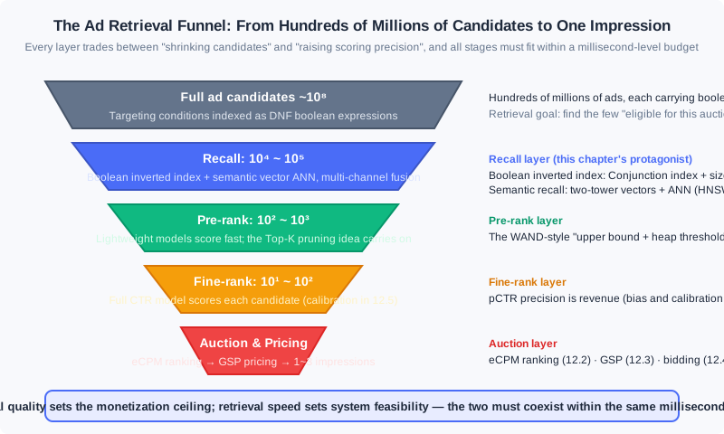
Three details in this figure deserve a stop. First, every layer is a trade between "shrinking candidates" and "raising scoring precision": the recall layer uses index structures (boolean inverted indexes, ANN vector indexes) to go from hundreds of millions to tens of thousands, at the cost of extremely coarse scoring (only "does it match" or "do the vectors look alike"); pre-ranking scores tens of thousands of candidates with lightweight models, engineering the WAND-style "rough upper bound + Top-K retention" idea; only fine-ranking applies the full CTR model to hundreds of candidates (its precision and calibration are covered in 12.5); finally the auction layer ranks by eCPM and prices by GSP. Second, upstream can never be compensated by downstream precision — an ad missed by the recall layer is invisible no matter how accurate fine-ranking is, so engineering prefers to over-recall (the "candidate superset" philosophy of the boolean index in the figure) and never lightly narrows the recall surface. Third, multi-channel recall is the norm: boolean targeting recall and semantic vector recall each produce one candidate stream in parallel, merged and deduplicated before flowing uniformly downstream — the two technologies of 12.9.3 and 12.9.4 are not substitutes but two intake pipes of the same funnel.
Compare this with recommender systems (the main line of the first half of this book): this funnel is nearly isomorphic to "recall → pre-ranking → fine-ranking → re-ranking" — ad systems and recommender systems share all the engineering wisdom at the retrieval layer, differing only at the funnel's end: recommendation optimizes user value, while advertising must additionally pass through a layer of bidding and mechanism design (the smart bidding of 12.4 decides how much advertisers are willing to pay for which candidates; the GSP of 12.3 decides how much is actually charged). Retrieval supplies the admission tickets for all of it.
⚠️ Common Mistakes in 12.9
| # | Mistake | Example | Why It's Wrong | Fix |
|---|---|---|---|---|
| 1 | Evaluating the boolean expression ad by ad | Iterating over hundreds of millions of ads on request arrival, judging each DNF one by one | The retrieval budget is only a few milliseconds; full evaluation necessarily times out — the two-layer index exists precisely for this | Build an inverted index over Conjunctions + a Conj→AD auxiliary index, and evaluate exactly only over the candidate superset |
| 2 | Ignoring size tier pruning, or counting into size | A request carrying only 2 labels queries all tiers with size=2 and above; using as an index key | When it can never be satisfied, so the whole tier can be skipped; does not enter keys and lives only on posting-list elements | size = the number of assignments containing "∈"; build the index tiered by size and prune tier by tier at query time |
| 3 | Moving a nonlinear fine-ranking function directly into the retrieval stage for pruning | Using a deep CTR model's scores as WAND upper bounds at retrieval | WAND's fast exclusion relies on "linear + non-negative weights" for the upper bounds to accumulate; nonlinear functions admit no accumulable | Use linear or generalized linear approximations at retrieval/pre-ranking; leave deep models to fine-ranking |
| 4 | After launching semantic recall, brute-force cosine over the whole corpus | Taking the dot product of the user vector with 1 million ad vectors per request | A full scan at 200 dimensions × millions takes tens of milliseconds, unacceptable under high concurrency | Deploy an ANN index (HNSW/IVF-PQ), accepting approximation in exchange for millisecond latency |
| 5 | Treating LSH/HKM as the contemporary mainstream | A new system picks LSH forest outright | LSH has a low recall ceiling and HKM has fixed search paths; engineering has replaced them with graph indexes and IVF-PQ | Modern choices favor HNSW/IVF-PQ; keep LSH for its "near points collide easily" intuition |
| 6 | Query expansion guided only by semantic similarity | A topic model expanding "laptop" to "laptop bags", ignoring monetization differences | Semantic relevance is not intent relevance, let alone high eCPM; over-generalization also harms search ad relevance | Use all three routes: collaborative filtering + topic models as fallback + historical eCPM performance data leading |
Chapter Summary
📌 Key Takeaways
| Concept | Key Points | Why It Matters |
|---|---|---|
| What makes ad retrieval special | Documents are DNF boolean expressions, not bags of words; queries may consist of hundreds of labels | Determines that ad retrieval cannot copy search-engine solutions and needs dedicated indexes and pruning |
| Boolean expression retrieval | Three-level decomposition DNF → Conjunction → Assignment; two-layer inverted index + size tier pruning; candidate superset + exact evaluation | The bedrock of millisecond retrieval over hundreds of millions of candidates, and one of the most core general technologies of auction advertising |
| WAND | Linear evaluation function + keyword upper bounds + min-heap threshold, exactly scoring only candidates that might enter the Top-K | Practical fast retrieval for extremely long queries (contextual targeting); the "rough upper bound + threshold positive feedback" idea carries into pre-ranking |
| Query expansion | Three routes combined: collaborative filtering (session × query matrix), topic models (semantic supplement), historical eCPM (directly aimed at revenue) | The traffic and revenue lever of search ads; over-generalization harming relevance is a hard boundary |
| Semantic recall | DSSM/two-tower: clicks as weak supervision, end-to-end semantic vectors, retrieval becomes nearest neighbor search | Resolves the generalization blind spot of keyword matching; the foundational form of contemporary recall technology |
| ANN evolution | LSH (intuitive origin) → vector quantization PQ/HKM → graph indexes NSW/HNSW; modern mainstream HNSW/IVF-PQ + multi-channel recall fusion | The engineering foundation of vector retrieval; vector quality matters more fundamentally than index choice |
❓ FAQ
Q1: Boolean retrieval or semantic recall — which do modern systems actually use?
Both, and in parallel. An advertiser's targeting conditions must be satisfied exactly (that is the contractual promise), so boolean inverted indexes are irreplaceable; semantic recall covers the "similar intent" traffic boolean logic cannot reach. Each produces one candidate stream, merged and deduplicated before entering ranking — i.e., multi-channel recall. Debating "which replaces which" is a pseudo-problem; the engineering difficulty lies in quotas and merging strategies for the multiple candidate streams.
Q2: How big is the practical impact of WAND's restriction to non-negative-weight linear functions?
Smaller than intuition suggests. Ranking models have long been dominated by generalized linear models (features × weights followed by a nonlinear link), and generalized linear scores can still be decomposed into accumulable linear terms, so the WAND framework applies directly. Even with deep models, linear/lightweight approximations can do Top-K screening at the pre-ranking layer — the divide-and-conquer idea does not depend on the specific model form.
Q3: What single principle suffices for ANN selection?
Vector quality before index choice. The gap between HNSW and IVF-PQ is at the level of engineering constants, while the sample and loss design of two-tower training (negative sampling, in-batch negatives, feature coverage) determines the ceiling of recall quality. A practical starting point for index selection: choose HNSW when memory is plentiful, IVF-PQ when candidates exceed hundreds of millions and memory is constrained, and leave the rest to benchmarks.
🔗 Connections to Other Chapters
- 12.2 (Billing Models and Core Metrics): retrieval's downstream endpoint is eCPM ranking, and the eCPM decomposition (pCTR × click value) directly defines "which candidates are eligible for admission"
- 12.3 (Auction Mechanisms): GSP pricing and the market reserve price act on the last layer of the retrieval funnel; retrieval quality determines how fierce the auction is
- 12.4 (Smart Bidding): the bid at the funnel's end decides what advertisers are willing to pay for; budget spend state in turn tightens upstream retrieval quotas
- 12.5 (Bias and Calibration): the calibration quality of fine-ranking pCTR affects eCPM ranking, and thereby the quota decision of "how much retrieval should recall"
- 12.7 (Online Allocation): traffic forecasting's "reverse index" and this chapter's ad retrieval inverted index are duals of each other — documents and queries swap roles, and one indexing technology serves two problems
Practice Problems
Work through all problems in order — they get progressively harder. Each has a complete solution you can reveal after trying it yourself.
Problem 12.9.1 — DNF Decomposition and Hit Evaluation 🟢 Easy
An ad's targeting conditions are: . Decompose it into a union of Conjunctions, write out each Conjunction's size (the number of assignments containing "∈"), and determine whether the following two requests hit this ad: (1) ; (2) .
Sample Input: Request (1) ; request (2) Sample Output: Decomposition , both Conjunctions have size 2; request (1) hits, request (2) does not
💡 Solution (click to reveal)
**Approach:** Split by "a segment joined by ∩ is one Conjunction, segments joined by ∪ are different Conjunctions", then check the request labels assignment by assignment.- Decomposition: , . Each contains 2 ∈ assignments, so both have size 2.
- Request (1): needs ✓ and ✓, satisfied → hit (in a DNF, one satisfied Conjunction suffices).
- Request (2): needs but the request has ✗; needs but the request has ✗ → no hit.
- Verify size pruning along the way: request (2) carries only 2 labels, so the size=2 tier is still queryable (); if the ad added one more ∈ assignment making size 3, the entire Conjunction could be excluded without any evaluation.
Key points:
- DNF hit condition: at least one Conjunction's assignments are all satisfied
- size counts assignments containing "∈"; is neither counted nor entered into index keys
Problem 12.9.2 — Simulating the Two-Layer Index Query 🟡 Medium
Using the 7 ads (–) and their Conjunction decompositions (–, where and ) from the figure in 12.9.3. The request is , size=3. Write out: (1) the candidate Conjunction set after querying all hit keys; (2) the candidate ad superset after taking the union through the second index layer; (3) the final hit list after exact evaluation, stating which ad is excluded and why.
Sample Input: Request labels Sample Output: Candidate Conjunctions ; candidate ads all 7 of ; final hits , with excluded
💡 Solution (click to reveal)
**Approach:** Query keys tier by tier → take the union at the second layer → exact evaluation, matching the figure's flow.- First-layer key lookup (all tiers with size ≤ 3 are queryable): size=2 tier, , , ; size=1 tier, . Candidate Conjunctions . (size=0) sits only under the special key and needs exact evaluation.
- Second-layer union: , , , , ; the union is — the candidate superset covers all ads.
- Exact evaluation: ( ✓), (: age=3 ✓, gender=Male ✓, geo=Beijing ∉{Guangdong} ✓), (: age ∈ {3,4} ✓), ( ✓), ( ✓), ( ✓). is excluded: needs gender=Female ✗, and needs geo ∉ {Beijing,Guangdong} but geo=Beijing ✗.
Key points:
- The size=1 is queried too — size pruning only skips tiers "with size greater than the label count", never small sizes
- The candidate superset may contain ads that ultimately do not hit (such as ); exact evaluation happens only on the superset — this is precisely the source of efficiency
Problem 12.9.3 — Walking Through WAND Pruning 🟡 Medium
A contextual targeting query contains 3 keywords, whose posting lists currently head at document IDs: , , . The keywords' contribution upper bounds are , , . The current min-heap is already full with results, and the heap-top score (the pruning threshold) is . Walk through the two steps of this WAND iteration, determine whether doc 5 gets exactly scored, and state the system's next action.
Sample Input: Posting-list heads ; upper bounds ; threshold Sample Output: The pivot stops at (accumulated upper bound ); the list heads of (doc 5) and the pivot list head (doc 9) disagree → doc 5 is not scored; advance some earlier list to doc 9 and start the next round
💡 Solution (click to reveal)
**Approach:** Step one sorts lists by head docID ascending; step two accumulates upper bounds to find the pivot, then compares the first and last list heads.- After sorting, the order is . Accumulating upper bounds: ; ; → the pivot is .
- Pivot check: the head docIDs of and are 5 and 9, not aligned → the current document (doc 5), even with full upper bounds, only sits on the two lists , so its true score upper bound is and it cannot enter the heap → doc 5 is pruned and not exactly scored.
- Next step: pick one of the earlier lists (say ) and skipto doc 9, returning to step 1; now heads align and the accumulation is ; if 's head also reaches 9, doc 9 deserves exact scoring.
Key points:
- What accumulates is the "upper bound", never the true score — if the upper bound falls short, never do exact scoring; this is the entire source of WAND's compute savings
- The heap-top threshold rises as the result set improves, making pruning ever harsher: the positive feedback is the deeper reason for WAND's efficiency
Problem 12.9.4 — The Recall Accounting of Random-Projection LSH 🔴 Hard
Use random projection for cosine LSH. The angle between two vectors is . (1) With a single hyperplane, what is the probability the two vectors land in the same bucket? (2) With hyperplanes forming an 8-bit signature (AND operation), what does the same-bucket probability become? (3) To boost recall, switch to LSH forest: independent signature groups take the union; what is the recall probability of "at least one group collides counts as a neighbor"? (4) With multi-probe instead, how many new signatures must a second-round query generate at and at ? Use this to explain the cost difference between the two recall-boosting schemes.
Sample Input: , , Sample Output: (1) ; (2) ; (3) ; (4) 8 at , 28 at
💡 Solution (click to reveal)
**Approach:** Substitute layer by layer into , the signature probability , the union recall , and the binomial .- (1) .
- (2) All 8 signature bits must match to share a bucket: . The AND operation makes buckets tiny and queries extremely fast, but a single signature's recall collapses.
- (3) At least one of signature groups collides: . Recall rises from 3.9% to 32.8%, at the cost of 10× index memory.
- (4) The number of new signatures flipping bits is : at , ; at , . Multi-probe adds no memory but launches multiple second-round retrievals per query; at the query count balloons quickly and the precision-recall trade-off is hard to control smoothly.
Key points:
- All three of LSH's recall-boosting means fundamentally trade something else for recall: forest trades memory, multi-probe trades query time, larger trades bucket precision
- The numbers expose LSH's limits — 90%+ recall would require astronomically many signature groups, which is one reason graph indexes replaced it
Problem 12.9.5 — Implementing the Two-Layer Boolean Inverted Index 🏆 Challenge
Implement the book example's full retrieval in Python: given the 7 Conjunctions (–) and the decomposition into 7 ads (–), implement build_index() (a size-tiered Conjunction inverted index + a Conj→AD auxiliary index, including the size=0 special key Z) and retrieve(query) (size pruning + key lookup + exact evaluation), and verify the output with four requests.
Sample Input: Requests , plus , ,
Sample Output: ['a1','a3','a4','a5','a6','a7']; ['a4','a5']; ['a2','a4','a5','a6']; ['a1','a4']
💡 Solution (click to reveal)
**Approach:** Model each assignment as an (attribute, value set, belong) triple; size counts only ∈ assignments; splits into two index keys; pure-∉ types hang on the special key Z and go through exact evaluation.# Each assignment: (attribute, value set, belong); belong=True means ∈, False means ∉
CONJUNCTIONS = {
"j1": [("age", {3}, True), ("geo", {"Beijing"}, True)],
"j2": [("age", {3}, True), ("gender", {"Female"}, True)],
"j3": [("age", {3}, True), ("gender", {"Male"}, True), ("geo", {"Guangdong"}, False)],
"j4": [("gender", {"Male"}, True), ("geo", {"Guangdong"}, True)],
"j5": [("age", {3, 4}, True)], # ← KEY LINE: one ∈ assignment, size=1
"j6": [("geo", {"Beijing", "Guangdong"}, False)], # ← KEY LINE: pure ∉ type, size=0
"j7": [("gender", {"Female"}, True), ("geo", {"Guangdong"}, True)],
}
ADS = {
"a1": ["j1", "j4"], "a2": ["j2", "j6"], "a3": ["j3", "j7"],
"a4": ["j5", "j4"], "a5": ["j6", "j5"], "a6": ["j6", "j1", "j7"],
"a7": ["j1", "j7"],
}
def build_index():
by_size, conj2ad = {}, {}
for c, assigns in CONJUNCTIONS.items():
k = sum(1 for _, _, b in assigns if b) # size = number of ∈ assignments
for attr, vals, b in assigns:
if b:
for v in vals: # age∈{3,4} splits into two keys
by_size.setdefault(k, {}).setdefault((attr, v), set()).add(c)
if k == 0: # pure ∉ types hang on the special key Z
by_size.setdefault(0, {}).setdefault("Z", set()).add(c)
for ad, cs in ADS.items():
if c in cs:
conj2ad.setdefault(c, []).append(ad)
return by_size, conj2ad
def holds(assigns, query):
for attr, vals, b in assigns:
q = query.get(attr)
if b and q not in vals:
return False
if not b and q in vals: # q not in the set means ∉ holds (including missing)
return False
return True
def retrieve(query, by_size, conj2ad):
conjs = set()
for k, posting in by_size.items():
if k > len(query): # ← KEY LINE: size pruning
continue
for key, cs in posting.items():
if not isinstance(key, tuple): # skip the special key Z
continue
attr, v = key
if query.get(attr) == v:
conjs |= cs
for c in by_size.get(0, {}).get("Z", set()): # size=0 goes through exact evaluation
if holds(CONJUNCTIONS[c], query):
conjs.add(c)
return sorted({ad for c in conjs
if holds(CONJUNCTIONS[c], query)
for ad in conj2ad[c]})
idx = build_index()
print(retrieve({"age": 3, "geo": "Beijing", "gender": "Male"}, *idx))
# ['a1', 'a3', 'a4', 'a5', 'a6', 'a7']
print(retrieve({"age": 4, "geo": "Beijing"}, *idx))
# ['a4', 'a5']
print(retrieve({"age": 3, "geo": "Shanghai", "gender": "Female"}, *idx))
# ['a2', 'a4', 'a5', 'a6']
print(retrieve({"gender": "Male", "geo": "Guangdong"}, *idx))
# ['a1', 'a4']
Note the third request: (geo ∉ {Beijing,Guangdong}, satisfied by geo=Shanghai) enters the candidates via exact evaluation under the Z key, dragging in the branches of and — this is exactly why the size=0 tier cannot rely on key lookup and must be evaluated exactly. The fourth request verifies the counterexample: is excluded by exact evaluation because geo=Guangdong ∈ {Guangdong}, even though both its and keys were hit (the request carries no age label; j3 entered the candidates via the gender key but was still blocked by the ∉ condition). Key points:
- Size pruning sits at
k > len(query): when the request lacks labels, entire tiers are skipped - exists only on posting-list elements (simplified here into the exact-evaluation stage) and never enters index keys
- Candidate superset → exact evaluation is the retrieval philosophy of "over-recall allowed, under-recall forbidden"
Data Processing and Trading
📝 Before You Continue: This chapter requires reading 12.2 (Billing Models and Core Metrics) first — data surcharges are settled on a CPM basis, and the eCPM frame of reference must be established beforehand; as well as 12.3 (Auction Mechanisms) — the RTB inquiry flow is the vehicle that data trading "hitches a ride" on. 12.4 (Smart Bidding) will show you where the labels ultimately flow: targeting and bidding features. 12.6 (Open-Loop and Closed-Loop Advertising) has already covered the identity-signal side — ATT/SKAN/Privacy Sandbox — while this chapter handles only the data compliance and trading side; the two are two sides of the same coin.
Precise targeting and aggressive bidding both rest on one premise: "you understand this user better than anyone else does." The user labels we have used repeatedly in earlier chapters — interests, intent, audience attributes — do not appear out of thin air: they come from the collection and processing of behavioral data, and in the programmatic trading market they are themselves a commodity that can be priced, bought, and sold. This chapter pulls the camera back from "how to serve ads" to "where does advertising's fuel come from": which data is genuinely valuable? Who turns raw logs into labels? How are labels priced and delivered? And — when you collect and trade user data, where are the legal and security boundaries?
The data industry originally existed to serve advertising, but today it has grown into a relatively independent industry. Understanding this chapter is not just understanding a supporting link of advertising — it is understanding the general craft of "how personalized systems turn behavior into assets."
After reading this chapter, you will be able to:
- Distinguish first-party, second-party, and third-party data, and judge the ownership and use of any given data item in advertising trading
- Rank various types of user behavioral data on the value ladder, and explain the logic behind two value rules
- Compare the responsibilities, business models, and product cases of first-party DMPs and third-party DMPs
- Describe the data trading mechanism relayed through the ADX: CPM pricing, delivery based on actual won impressions, and the economic problem of "data prices shifting into traffic prices"
- Master the basic principles of privacy protection, the ideas of quasi-identifiers and K-anonymity, identify data security risks on both the supply and demand sides of programmatic trading, and complete 5 tiered practice problems
12.10.0 Three-Party Data: The Fuel of Targeting and Bidding
Every decision an ad system makes — which candidates to retrieve, how high to estimate the click rate, how much to bid — is essentially "trading data for judgment." The auction mechanisms of 12.3 gave traffic a market price, and what makes the same traffic carry a different price in the eyes of different DSPs is precisely the data each of them holds. So the collection, processing, and trading of data is just as important as the ad-serving technology itself.
User data used in advertising falls into three classes by source. First-party data comes from the advertiser: their own CRM, order records, and website visitor behavior. Second-party data comes from the advertising platform: behavioral data generated by users on the media or platform and held by the platform itself. Third-party data comes from data providers that do not directly participate in ad trading — small and mid-sized media, membership systems, and various data companies. Under the ad network model, second-party data was the main guide for delivery; in the era of real-time bidding (12.3), the game changed: first-party data could be activated, and the third-party processing and trading of data developed along with it.
The three classes of data are not equal in standing. First-party data is generally small in volume, yet it is the soul of all data — it relates directly to your business, has the clearest semantics, and sits closest to conversion. Building on first-party data and making good use of second-party and third-party data is the most important methodology of the RTB era. The ecosystem diagram below is this chapter's roadmap: data departs from the three source classes, is processed by DMPs into labels, is traded through the ADX and attached to every bid request, ultimately becomes ammunition for targeting and bidding in the DSP, and delivery outcomes flow back as new data — closing the loop.
🧠 Mental Model: The Oil Refinery
Picture the data ecosystem as the petroleum industry. Raw behavioral logs are crude oil — buried underground, unable to drive anything directly; the DMP is the refinery — fractionating crude into gasoline and diesel (standardized user labels); the ADX is the gas station and fuel meter — selling refined fuel by the liter (labels attached to traffic on a CPM basis); the DSP is the engine — burning fuel to produce power (targeting and bidding); and the exhaust emitted at the end (conversion data) is recovered and refined again — the loop's feedstock never runs out. Remember one contrast: your own oilfield (first-party data) has modest output, but the best quality and ownership; the wholesale market (third-party data) is abundant and cheap, but of uneven quality.
12.10.1 Valuable Data Sources
Data is the core of the precision advertising market, but not all data is worth collecting and processing. Which data directly contributes to the advertising business? We go through each class and provide a framework for judging value.
User identifiers. Determining which behaviors come from the same user is the most easily underestimated problem. A stable user identity is like the 1 in front of a string of 0s: no matter how much behavioral data you can obtain, if you cannot link it to the person in the delivery system, the data is useless. The foundational solution of the browser era was the cookie — although multiple browsers, expiration, and users actively clearing them all break long-term consistency, recent behavior is what matters most in advertising anyway, so cookies remained a widely adopted industry solution; if the domain operating the ads also provides permanent identity services such as email or social networking, expired cookies can be recovered through the permanent identity. Mobile diverged: iOS uses the advertising-specific identifier IDFA, similar in nature to a cookie; Android has no dedicated ad ID, so device identifiers such as the Android ID or IMEI are generally used. A high-quality user identifier is itself a valuable asset that can be exchanged and sold in the marketplace — we will pick this thread up again in the modern notes of 12.10.2.
User behavior. The industry broadly agrees that the online behaviors worth collecting at scale, with a clear effect on targeting, include: conversions, pre-conversions, search ad clicks, display ad clicks, search clicks, searches, shares, page views, ad views, and so on. By their effectiveness for performance advertising, they fall into four tiers:
- Decision behaviors: conversions and pre-conversions — both happen on the advertiser's own site. In e-commerce, a conversion corresponds to the final order, while a pre-conversion covers the preparatory actions before ordering: searching, browsing, comparing prices, adding to cart, and so on. These behaviors point most clearly at intent, carry the highest value, and are also the hardest for supply-side or ad platforms to obtain; using them for retargeting or personalized retargeting is the most direct exploitation. The volume is not large, but they cannot be ignored.
- Active behaviors: ad clicks, searches, search clicks — produced actively by the user under explicit intent, rich in information. Ad clicks are too few in number to serve as the main source of targeting; search is the most important active behavior obtainable at scale, and deserves special mining.
- Semi-active behaviors: shares, page views — arising from content consumption with weaker purpose; they capture the domain of interest but with limited content precision. Their guidance value is limited, yet their volume is the largest of all behavior classes.
- Passive behaviors: ad views — strictly speaking not a behavioral basis for targeting, but their frequency is negatively correlated with clicks on ads of the corresponding category, so they remain usable in behavioral targeting models.
There are two basic rules for judging value. First, as the user's active intent rises, the value of the behavioral data increases. Second, the closer a behavior is to conversion, the more precise its guidance for performance advertising. But there is one easily overlooked caveat here: the fundamental purpose of advertising is to "reach potential users at low cost." Behaviors close to conversion are more precise because that population already stands at the final stage of the decision — in other words, they are less and less "potential users." Targeting solely by conversion ROI collapses coverage to the very bottom of the funnel. The right approach is to balance effectiveness and coverage according to the advertiser's audience-reach goals.
Demographic attributes. Commonly used targeting labels, but limited in source: generally only services that can be bound to real-name identities can obtain them directly. Predicting demographic attributes from behavioral data is a common practice, but accuracy is limited and labeled calibration data is still needed for training. Certain special signals can actually yield accurate judgments — for example, the voice signals recorded by voice services can distinguish male from female fairly reliably.
Geographic location. Its usefulness changes drastically with precision. IP mapping only reaches city level, which is already valuable for many campaigns; in mobile environments GPS or cellular positioning can reach a few hundred meters of accuracy, capturing users' offline store-visit interests and making precise location targeting possible for local advertisers such as restaurants.
Social relationships. Social connections imply the reasonable inference of "similar interests," which can be used for smoothing user interests: when a user's behavioral data is insufficient for precise targeting, one can borrow the behaviors and interests of the user's social-network friends — a person whose Weibo friends mostly love football probably loves football too. Such smoothing applies only to long-term stable interests, not to short-term purchase interests; hence strong-tie social networks have an advantage over weak-tie ones.
Device information. Mobile devices can supply far richer data than PCs: the installed app list, device model, gyroscope readings, even status information such as battery level — all very helpful for identifying usage contexts. Deep processing of device information has particular significance for mobile advertising.
Analysis: There is no single universal "ranking" across the six data classes, because value depends on the use: in performance campaigns, decision behaviors overwhelm everything; brand-awareness campaigns should precisely avoid the conversion-adjacent population, and the large volume of semi-active behaviors becomes the friend of coverage. The truly universal judgment framework is those two rules (active intent, distance from conversion) plus one reverse reminder (too close to conversion means no longer a potential user). Before collecting and processing, run the data through this framework once: whose goal does this data serve?
12.10.2 The Data Management Platform (DMP)
Given raw data, who refines it into usable audience labels? Products that organize and process data into directly usable information and support monetization are collectively called Data Management Platforms (DMPs). In the market, DMPs come in two settings — first-party and third-party: the technical steps are basically the same, but the product direction and business model differ greatly.
First, a technical detail left over from 12.10.0: cookie mapping. When the advertising business domain differs from the domain holding the permanent identity, and with the latter's consent, mapping technology can align user identities across the two — this is the infrastructure of data integration and trading, and the star topology of data trading described later is optimized precisely around it.
First-party DMP: data hosting and processing service. For advertisers or media without technical accumulation, building a dedicated team for data processing is not worthwhile, so products specializing in this business emerged. They have two core functions: one is providing audience targeting capabilities for websites (media or advertiser sites), processing both general-purpose labels and custom audiences according to the website's own label taxonomy; the other is letting advertisers conveniently connect their data with ad purchasing channels. The value of the latter can be understood this way: an advertiser doing external retargeting needs to notify ad platforms of its user set — if every platform installed tracking code on the site, first the pages would grow ever heavier, and second visitor accumulation would take weeks at a time, making retargeting inefficient. Having the DMP uniformly handle user accumulation and segmentation, then pass segments to ad platforms through data interfaces, solves both problems at once.
The first-party DMP collects and processes data according to the needs of the data provider (DP), charging the DP a service fee. It is a data hosting and processing service that does not aim to monetize the data itself: it must never treat client data as its own property for secondary monetization, nor mix data across different DPs — this is the bottom line of this product's business model. Its clients are mostly mid-to-large media and advertisers; capable advertisers can also build their own DMP.
Third-party DMP: the data trading platform. Its main product function is aggregating online user behavioral data from various sources, processing it into valuable user labels, and monetizing by selling the labels, with revenue shared proportionally back to the data providers. It often also carries the processing capabilities of a first-party DMP, but the key difference is that a data trading platform builds its label taxonomy and processes data according to its own logic, not the media's needs — hence it offers its product from the third-party data standpoint and is called a third-party DMP. Its DPs are mainly small and mid-sized media and data owners — players with plenty of data for whom standalone monetization is not worthwhile.
Analysis: The two DMP business models side by side. First-party DMP: sells a "service" — clients pay hosting and processing fees, data ownership stays with the client, and the product emphasizes flexible integration and custom labels. Third-party DMP: sells "data" — processes under its own label taxonomy and sells to DSPs, sharing revenue with DPs; the product emphasizes label coverage and category operations. The former follows a to-B service logic — stable profits but a low ceiling; the latter follows a commodity-circulation logic — large upside but full responsibility for data quality and compliance. This divide determines the trajectory of all the product cases that follow.
Product cases. The international market once had three representatives. BlueKai was the archetypal third-party DMP: it built its Data Exchange database in 2008, on one side having small and mid-sized websites contribute traffic and membership data, and on the other processing it and selling it to advertisers; it insisted on not providing media bidding/purchasing services in order to stay neutral and integrate with multiple DSPs — this "independent DMP" route was highly successful for a time, with over 300 million active users and 80% of the top 20 ad networks and portals using its data; in 2014 it was acquired by Oracle for 400 million dollars. Its label taxonomy was open-ended: Intent (recent search terms indicating demand, over 1.6 billion users), B2B (from Bizo), Past Purchase (Addthis, Alliant), Geo/Demo (blending multiple sources such as Bizo, Datalogix, and Expedia), Interest/Lifestyle, and more, continuously expanded by source and market demand — fine-grained categories like "people interested in P&G shampoo" or "people planning a trip to Japan" were highly meaningful to performance advertisers and sold at a premium. AudienceScience represented another path: it proposed the concept of audience targeting earliest, mainly providing first-party DMP services (e.g., processing finance and sports user labels for The New York Times), while also running its own performance ad network for monetization — it did not sell labels directly; instead it shared the revenue created by labels with the media that provided the data, because "after deducting revenue shares, the profit margin of data processing alone was too small, and running one's own ad network offered larger arbitrage." It shut down in May 2017, which also reflected that standalone data services had rather limited scale and profitability. TalkingData was the representative in the Chinese market: it entered through an app analytics tool, accumulated massive independent-device data, and then launched its marketing cloud, MarketingCloud, with features including user ID mapping and management (linking the same user across ID systems such as CRM, offline stores, online browsing, and official accounts), an open third-party label library (over 800 fine-grained dimensions), geofenced target audiences, and marketing process monitoring and management — its business model was closer to a first-party DMP, making it a pioneer of the "data-driven marketing automation" direction.
💡 Modern Notes (2026): The cases above read like a documentary from "the pre-smartphone era." Third-party cookies have been blocked in Safari (ITP) and Firefox, and Chrome has moved to a user-choice model — cookie mapping as industry infrastructure has in fact ended, and the identity-signal degradation described in 12.6 is precisely its final act. The replacement is a new suite of first-party data infrastructure: the CDP (Customer Data Platform) unifies data from a brand's own touchpoints (website, app, mini-program, CRM) into persistent customer profiles, replacing most scenarios of the old first-party DMP; cross-domain identity relies on Unified ID 2.0 (UID2) — an open identity framework led by The Trade Desk, rooted in hashed email addresses/phone numbers — and on the first-party IDs of giants like Amazon built on their own account systems. The former independent DMPs (BlueKai, LiveRamp, etc.) were either absorbed through M&A or transformed into identity and data collaboration service providers. The business-model lessons in the old book have not aged: data capability is concentrating in the hands of whoever holds the logged-in state, and neutral third-party data is being squeezed out by compliance and technology alike.
12.10.3 The Basic Process of Data Trading
The labels are processed — how to sell them? Data trading is generally completed with the ADX or SSP as the intermediary: the DMP's various user labels are delivered to the ADX in batch transmission and sold to DSPs as the ADX's auxiliary product. Labels are generally priced on a CPM basis: if a DSP chooses to buy a certain label, then during ad inquiries the ADX passes that request's user labels to the DSP along with the request, and the final charge is the DSP's actually won impressions × the CPM price as the data surcharge.
Conducting data trading piggybacked on ad trading is far more sensible than direct DMP-to-DSP trading, for four reasons:
- Transmission cost. Data volumes can be huge, and the transmission cost of direct connections is non-negligible; attaching user labels to ad requests brings almost no additional serving overhead — total transmission cost reduces to the single hop from DMP to ADX.
- Star topology. Every DSP and data provider only needs to do cookie mapping with the ADX, and the ADX's user reach far exceeds that of any single DSP or DMP — minimizing the data loss caused by mapping.
- Partial trading. A DSP rarely needs all of a DMP's data; by transmitting data within the trading process, the DSP can freely limit the scope it needs — a DSP serving only Shanghai, once it selects the Shanghai region, will only receive Shanghai data.
- Natural billing. The ADX happens to stand between buyer and seller, incidentally completing data-usage monitoring and billing — it is already the party counting the money.
🧠 Mental Model: Tap Water and the Water Meter
Data trading is like water supply. DMP-to-DSP direct trading is like every household digging its own well and laying its own pipes — N pipelines, each requiring settlement, costs exploding; trading through the ADX is like a water utility laying one unified pipe network (batch transmission + star mapping), with the meter installed at the ADX (each won impression × CPM), paying by usage. Even better is "partial trading": you can order only Shanghai's water (limit the label scope) without buying the entire reservoir. But tap water and mineral water differ in one fundamental way: the same data can be resold to many buyers, and everyone is drinking from the same aquifer — which is exactly the trouble discussed below.
The uniqueness of data as an information commodity lies in two points: it can be resold (like software in this respect); but unlike software, all users of the same data face the same pool of users, so a game-theoretic relationship exists among them. From this arise two deep problems.
First, reselling data causes data prices to shift into traffic prices. Consider an example: a DMP knows a certain user is a golf enthusiast and sells this information to one DSP — that DSP uses it to earn high returns and can naturally afford a high data procurement price. But if the DMP sells it to multiple DSPs, when these DSPs target the same user they will inevitably bid up the traffic cost against each other, diluting the returns gained from this data and indirectly depressing the data's monetization price. The more it is sold, the more each copy's value is diluted by bidding — profit shifts from "data dividend" to "traffic price." Second, under resale data cannot be sold by auction. The online advertising market owes its large gains in customer count and monetization precisely to the auction model (12.3), so we naturally hope data can be auctioned too. The direction is limited-quantity selling: each piece of information should be offered to only a limited few buyers within a given time window, which is the only way an auction model could develop while protecting data providers' interests. But exactly how many buyers to limit, and how to design the auction mechanism, remain open questions.
Analysis: The design essence of this mechanism is "hitching a ride": embedding the trading of a new commodity (labels) into an already mature market (RTB), reusing its transmission channels, identity mapping, billing, and monitoring facilities, at near-zero marginal cost. Compared with the inquiry flow of 12.3, data trading adds not a single extra round trip. The limitation comes from the same place: data value is unverifiable before delivery (only an A/B test tells whether the label is worth it), so pricing can only be a one-size-fits-all CPM; add the dilution effect of resale, and the market ultimately moved toward the compliant form described in the next section.
💡 Modern Notes (2026): Trading plaintext audience segments has shrunk dramatically in mature markets, and the mainstream compliant form is the Data Clean Room: advertisers import their first-party data and platforms import behavioral data into a controlled environment, where matching, overlap analysis, and effectiveness measurement are done under the premise that neither side can see the other's raw records — only aggregated reports are output (often with differential-privacy noise added), never raw audience segments. Google Ads Data Hub, Amazon Marketing Cloud, Meta's advanced analytics tools, and neutral offerings such as LiveRamp all belong to this form. The differential privacy and GDPR/PIPL compliance requirements of 12.10.4 are precisely the technical foundation of the clean room; together with UID2, it forms the new paradigm of data collaboration in the 2020s — data usable but not visible.
12.10.4 Privacy Protection and Data Security
Advertising is a typical personalized system: targeting depends on user behavioral data, and the trading market is busy buying and selling that data. So two classes of security problems must be considered together — user privacy (whether personal information leaks), and the commercial data security of data owners (whether an advertiser's key data gets exploited by the platform or competitors).
The real difficulty of privacy is subtler than "bulk leakage." Beyond mass leaks of user records, the bigger challenge is privacy prying aimed at acquaintances: the pryer already holds some background information about the target and uses it to dig out more privacy. Such attacks may combine human and machine effort and are insensitive to cost, hence the most damaging — there was a real case of someone pinpointing another person's home address on social media by analyzing posts and photos.
Against this background, the industry converged on several consensus principles of privacy protection:
- Strictly avoid using personally identifiable information (PII) — ID numbers, phone numbers, email addresses, home addresses, and the like, which can conveniently locate a specific person, must be protected unconditionally and strictly. The prevailing understanding at the time was that user identifiers such as cookies and IMEIs do not conveniently identify a person and are not PII (an understanding that needs revision under today's legal environment — see the modern notes).
- Users have the right to stop being tracked. Behaviorally targeted ads should give a clear notice (such as the AdChoices mark in the top-right corner of the creative), and users can use an Opt-Out action to notify the system to stop recording and using their behavioral data — handing the decision of whether to accept personalized advertising to the user.
- User behavioral data should not be retained long-term. Long retention adds little targeting value while magnifying leak risk; expired data with no direct business relevance should no longer be stored.
- Strict permission assignment and minimal data access. Sampled, anonymized data subsets for debugging; raw data accessible in production only through special keys; even developers, and management, should have no data access rights.
Quasi-identifiers: is removing PII enough? Take this record: "age 36; works in a certain office building in Shanghai; male; test engineer; hobby badminton; monthly salary 15,000 yuan" — name and phone number are hidden, but his friend can still identify him at a glance via the combination of "age + workplace + job title + hobby," and thereby read the privacy of "monthly salary." Such information — individually unidentifying but capable of locating a person in combination — is called a quasi-identifier. The countermeasure is generalization: generalize "36 years old" to "30–40 years old," "a certain building" to "Shanghai" — if, after generalization, every group of quasi-identifier instances in the dataset has K records identical to it, K-anonymity is achieved. With K chosen reasonably, leakage risk drops significantly.
Sparse behavioral data: K-anonymity cannot save personalized systems. A personalized system's description of a user includes a large amount of behavioral data, and behavioral data is extremely sparse — the behaviors of any two users are almost never identical, so K-anonymity has no foothold. The risk has real precedents: the famous Netflix Prize recommendation competition released a dataset from which PII had been removed and K-anonymity applied, but viewing histories and ratings were left untouched — researchers found that by simply matching these sparse behavioral data against public data such as IMDb, users could be re-identified with fairly high accuracy; earlier, users had already been identified from others' viewing records (including some films on homosexual themes). This line of research greatly raised industry awareness of privacy and spurred the study of differential privacy: modifying the dataset to a certain degree so as to minimize leakage risk with as little loss of query accuracy as possible (Apple claimed to have integrated the technique in iOS 10). Frankly, the risk of sparse behavioral data still has no mature solution to this day — it is the sword of Damocles hanging over the large-scale use of behavioral data, and data trading and disclosure must treat it with reverence.
Data security in programmatic trading. RTB brings the data of both the supply and demand sides together in a single transaction, and this double-edged sword cuts on both sides.
Supply-side data security: the ADX broadcasts every impression's URL and cookie to the bidding DSPs, so in theory a DSP could surveil a media's user behavior at scale — a malicious DSP bids an extremely low price on all requests, aiming not to win traffic but to collect user behavior on the media. Fortunately the actual harm is controllable: due to bandwidth limits, the ADX performs inquiry optimization (sending inquiries only to the DSPs most likely to win), so a data-collecting DSP would ideally be shut out of most inquiries.
Demand-side data security: the more serious side. After custom labels were introduced into RTB, the advertiser's first-party data is also exposed in the trading process. Imagine two English-education advertisers both doing retargeting through a DSP: each one's visitor set is the advertiser's most commercially valuable private data, yet the DSP, ADX, and media may all obtain them during the RTB process. If the DSP wants to create a more intense bidding environment, it can merge the two advertisers' visitor sets, tag them with a vague label like "English-education audience," and attract both sides to bid — in effect trafficking in visitor sets between competitors, and in a very covert way. The fiercer the bidding, the more profit that originally belonged to the advertisers shifts to other links of the market. This issue determines whether advertisers dare to procure via RTB with confidence, and the market's current attention and solutions are both inadequate — when using first-party data with powerful ad platforms, advertisers must be especially vigilant about data security (the modern countermeasure is exactly the clean room in the 12.10.3 notes: visitor matching completed in an environment where neither side sees the other's records).
GDPR: the legislative benchmark of privacy protection. In April 2016 the European Parliament passed the General Data Protection Regulation (GDPR), effective May 2018, binding any organization that collects, transmits, retains, or processes personal information of EU member-state residents. Three key points. First, it explicitly lists sensitive data — racial or ethnic origin, political opinions, religious/philosophical beliefs, trade-union membership, health/sex life/sexual orientation, genetic data, and biometric data (the last two being reasonable extensions for the new era). Second, processing must rest on explicit consent, and consent language must state clearly what information is collected and how it is stored and used — vague clauses are no longer allowed. Third, it grants users four rights — the right of data access (to learn how a company uses one's data), the right to be forgotten (to demand deletion of collected data), the right to restriction of processing (to forbid use in marketing or disclosure to third parties), and the right to data portability (to take one's personal data along when leaving a platform).
💡 Modern Notes (2026): The precise upper bound of GDPR penalties is "the higher of 20 million euros or 4% of global annual turnover" — that is the actual teeth of "the strictest in history," far more deterrent than a vague "tens of millions of euros." The book's original criticisms of GDPR (execution standards left vague, enterprises themselves unable to explain how data is used in the deep learning era, retrofit costs favoring oligopolies) remain worth debating, but history has delivered its verdict: legislation worldwide followed GDPR, and China's Personal Information Protection Law (PIPL) took effect in November 2021, establishing principles such as informed consent, minimal necessity, and withdrawable consent, and likewise distinguishing sensitive personal information; cookie-type identifiers have been brought into the scope of personal information across multiple jurisdictions — the 8.4-era belief that "cookies are not PII" is now history. As for how the signal-side privacy infrastructure — ATT/SKAN/Privacy Sandbox — adapts in delivery, 12.6 covered it in detail and this chapter does not repeat it; one-sentence cross-link: 12.6 covers "how to advertise after signals weaken," this chapter covers "how data is governed in trading and compliance."
12.10.5 Closing: The Data Monetization Loop
Fit this chapter's parts back into one picture (recall the ecosystem diagram of 12.10.0):
Data sources → DMP processing → trading → DSP application → performance flowing back.
- Data sources: first-party (advertisers, the soul), second-party (ad platforms), third-party (other data providers), ranked by "active intent × distance from conversion";
- DMP processing: first-party DMPs do hosting and custom processing for a service fee; third-party DMPs process labels under their own logic and sell to monetize, sharing revenue with data sources — the modern form evolved into the identity infrastructure of CDP + UID2/first-party IDs;
- Trading: labels are ingested into the ADX in bulk, attached to bid requests and priced on CPM, delivered on the DSP's actually won impressions — the modern form evolved into the clean room's "usable but not visible" collaboration;
- DSP application: labels enter targeting and bidding (12.3's auctions, 12.4's smart bidding), with the purchase scope limited on demand;
- Performance flowing back: conversion data flows back to the data-source side, becoming the feedstock of the next round of processing — 12.6's closed-loop measurement is the modern incarnation of this return flow.
A few engineering and business judgments worth taking away: the value of data lies not in quantity but in its match with the business goal — performance advertising wants decision behaviors, brand reach wants coverage; the market design of data trading is far from complete — price dilution from resale and the absence of an auction mechanism are textbook-grade open problems; and privacy and data security are not a compliance cost but the pressure-bearing wall of this fuel system — the Netflix re-identification and visitor-set trafficking cases remind us that any crack in that wall costs the entire ecosystem its trust.
⚠️ Common Mistakes in 12.10
| # | Mistake | Example | Why It's Wrong | Fix |
|---|---|---|---|---|
| 1 | Targeting only with behaviors close to conversion | Using only purchasers/cart-adders as the lookalike seed | That population is already at the end of the decision funnel and is no longer "potential users"; coverage collapses, violating the fundamental purpose of "reaching potential users at low cost" | Balance ROI and coverage by the advertiser's reach goal: performance campaigns weight decision behaviors, brand campaigns turn to the volume of semi-active behaviors for coverage |
| 2 | Treating the first-party DMP as a data monetizer | The DMP privately selling client audience segments to other buyers, or mixing data across clients to build new labels | A first-party DMP is a data hosting and processing service; secondary monetization of client data destroys the business model and trust outright | Write data ownership into contracts; monetization appears only in the third-party DMP model, and must share revenue with data providers |
| 3 | Believing that removing PII eliminates privacy risk | Publishing de-identified behavioral details externally | Quasi-identifier combinations can locate individuals; sparse behavioral data is nearly impossible to K-anonymize (the Netflix re-identification case) | Generalize quasi-identifiers and aggregate before output; route detail data through a clean room, outputting only aggregated results with differential privacy added |
| 4 | Billing the data surcharge on inquiries rather than wins | The DSP charged for every labeled request received | Data trading's delivery basis is "actually won impressions × CPM"; billing on inquiries makes the DSP pay for traffic it never bought | Reconcile against the ADX's win logs; the scope limits of partial trading (region/category) must also be checked into the billing |
| 5 | Ignoring demand-side data security | Opening retargeting audience segments directly to DSP custom labels with no isolation clauses | The DSP/ADX may merge visitor sets and resell them to competitors, engineering bidding that inflates traffic costs and shifting profit to the market | Sign data-use restriction clauses; do visitor matching in a clean room; monitor abnormal drift in win rate and traffic cost |
| 6 | Copying cookie-era solutions into 2026 | Designing label distribution that depends on third-party cookie mapping, or claiming cookies are not personal information | Third-party cookies are dead in Safari/Firefox and Chrome has moved to user choice; multiple jurisdictions have brought identifiers into the scope of personal information | First-party data goes through CDP + UID2/first-party IDs; cross-party collaboration goes through clean rooms; compliance follows the GDPR/PIPL standard |
Chapter Summary
📌 Key Takeaways
| Concept | Key Points | Why It Matters |
|---|---|---|
| Three-party data | First-party = advertisers (the soul), second-party = ad platforms, third-party = other data providers; RTB-era methodology: build on first-party data and use second- and third-party data well | The source of all targeting and bidding differences, and the basis for judging data asset ownership |
| Data value ranking | Decision > active > semi-active > passive; two rules: stronger active intent means higher value, closer to conversion means more precise guidance; reverse reminder: proximity to conversion means losing "potential" status | The investment judgment framework before collecting and processing data |
| Two DMP models | First-party DMP: hosting and processing for a service fee, never secondary monetization; third-party DMP (data trading platform): process and sell under its own logic, sharing revenue with DPs; modern evolution: CDP + UID2/first-party IDs | Understanding the genealogy of data-product business models and 2026 first-party data infrastructure |
| Data trading mechanism | Relay through the ADX: bulk label transfer, attached to inquiry requests, surcharge billed as actually won impressions × CPM; four benefits: transmission cost, star mapping, partial trading, natural billing; open problems: resale shifts price into traffic, auction model unexplored | The standard form of label circulation in programmatic markets and its economic limitations |
| Privacy protection | Four principles (avoid PII / Opt-Out / no long-term retention / minimal access); quasi-identifiers and K-anonymity; no mature solution for sparse behavioral data (Netflix case); differential privacy | The safety bottom line of data use in personalized systems, and the technical root of the clean room |
| Trading data security | Supply side: malicious low-bid DSPs surveilling, mitigated by inquiry optimization; demand side: visitor sets merged and resold, profit shifting to the market — more critical than the supply side | Determines whether advertisers dare to plug first-party data into programmatic trading |
| GDPR / PIPL | GDPR: sensitive data list, explicit consent, four rights (access / erasure / restriction / portability), penalty cap max(€20M, 4% of global revenue); PIPL effective 2021 | The two great foundations of global data compliance, unavoidable for multi-jurisdiction businesses |
❓ FAQ
Q1: Is the era of the third-party DMP completely over?
Trading of plaintext audience segments has indeed shrunk, but the need to "aggregate data from many sources and process it into commercially usable labels" has not disappeared — it changed form: from independent DMPs to platform-internal data markets (rooted in the platform's own identity system), clean room data collaboration, and audience solutions built on open identities like UID2. The old model died from collapsing identity infrastructure and compliance pressure; what was learned — label taxonomy design, data quality operations, revenue-sharing mechanisms — is all reusable in the new forms.
Q2: What does "data prices shifting into traffic prices" mean for the data buyer?
It means the dividend of "buying data" automatically dilutes with competition: when multiple DSPs hold the same label and bid on the same traffic, the data advantage converts into a higher win price, and profit shifts from the data side to the traffic side. The buyer's countermeasure is to use data on "cross combinations others don't have" (the more exclusive the better), and to keep validating the data's marginal contribution with incremental experiments, rather than paying for mere possession.
Q3: Should an advertiser build its own DMP/CDP or use an external service?
Depends on data scale and team. With large data volumes, an engineering team, and data as core competitiveness (large retail, finance), building your own gives the best control; otherwise use an external first-party DMP/CDP service, but hold two bottom lines: the contract must state data ownership and use restrictions, and the provider must never be allowed to mix your data with other clients' or monetize it a second time. Either way, high-value audience collaboration such as visitor matching should always go through a clean room.
🔗 Connections to Other Chapters
- 12.1 (Panorama and Ecosystem): this chapter's data loop is embedded in the full advertising ecosystem — the supply-side answer to "where do targeting and bidding come from"
- 12.2 (Billing Models and Core Metrics): the CPM basis of the data surcharge and the eCPM definitions rest entirely on 12.2
- 12.3 / 12.4 (Auction Mechanisms / Smart Bidding): after labels are traded through the ADX, they ultimately enter these two chapters' decision engines as targeting conditions and bidding features
- 12.6 (Open-Loop and Closed-Loop Advertising): the signal-side ATT/SKAN/Privacy Sandbox is covered there, while this chapter handles the data compliance and trading side; the performance-return loop is modernized in 12.6's closed-loop measurement
- 12.7 (Online Allocation): traffic forecasting aggregates traffic by label combinations — the quality of the label taxonomy directly determines forecasting and allocation accuracy
Practice Problems
Work through all problems in order — they get progressively harder. Each has a complete solution you can reveal after trying it yourself.
Problem 12.10.1 — Ranking Behavioral Data by Value Tier 🟢 Easy
Classify the following online behaviors into the four tiers "decision / active / semi-active / passive," and identify which one is "the most important active behavior obtainable at scale":
e-commerce order, add to cart, ad click, share, page view, search, search click, ad view, price comparison before ordering
Sample Input: the 9 behaviors above Sample Output: Decision: {e-commerce order, add to cart, price comparison before ordering}; Active: {ad click, search, search click}; Semi-active: {share, page view}; Passive: {ad view}; largest-volume active behavior: search
💡 Solution (click to reveal)
**Approach:** Decision behaviors = conversion + pre-conversion, all occurring on the advertiser's site; active behaviors = clicks and searches under explicit intent; semi-active behaviors = weak-purpose content consumption; passive behaviors = the ad exposure itself.- The e-commerce order is a conversion; adding to cart and comparing prices before ordering are typical pre-conversions — all three are decision behaviors.
- Ad clicks, searches, and search clicks are all active behaviors; among them ad clicks are too few in volume, and only search is "the most important active behavior obtainable at scale."
- Shares and page views are semi-active behaviors; ad views are passive behaviors — their frequency is negatively correlated with clicks on similar ads, and they remain usable for modeling.
Key points:
- Pre-conversions (price comparison, cart addition) belong to decision behaviors — they occur on the advertiser's site with clear intent
- The judgment criteria are "strength of active intent × distance from conversion," not data volume
Problem 12.10.2 — Computing the Data Trading Surcharge 🟢 Easy
A DSP buys the "parent-and-baby audience" label from an ADX at a CPM price of ¥2.50. This month all impressions it won that carried this label total 120,000 (all matching the label's definition).
(a) What is this month's data surcharge? (b) If these impressions bring 480 conversions, what is the data cost per conversion? (c) Next month the DSP serves only Shanghai; under the "partial trading" rule it receives only 90,000 won impressions matching the label. What does the surcharge become? Which of the four benefits of data trading does this illustrate?
Sample Input: label CPM ¥2.50; won impressions {120000, 90000}; conversions 480 Sample Output: (a) ¥300 (b) ¥0.625/conversion (c) ¥225; partial trading
💡 Solution (click to reveal)
**Approach:** Delivery basis = actually won impressions × CPM price.- (a) mille, , surcharge ¥300.
- (b) , data cost per conversion ¥0.625. This number feeds directly into ROI accounting: purchasing pays off only when the incremental conversion value the label brings exceeds ¥0.625 per conversion.
- (c) , , surcharge ¥225. The DSP bought data for the single region of Shanghai and is billed only on wins within that scope — precisely the benefit of "partial trading": the DSP freely limits the data scope it needs and pays nothing for data it cannot use.
Key points:
- The billing base is "actually won impressions," not the number of inquiry requests (contrast Common Mistakes #4)
- Partial trading plus win-based billing together form the data trade's protection for the buyer
Problem 12.10.3 — Three-Party Data Ownership and DMP Selection 🟡 Medium
Determine the ownership class (first-/second-/third-party) of the data in each of the three scenarios below, and for each scenario pick the most suitable data product route (A: first-party DMP/CDP self-built or hosted; B: connect to a third-party DMP/data trading platform; C: a combination of both), with reasons.
- The New York Times: owns massive first-party users and online data, but its core business is neither advertising nor data processing.
- A small online clothing shop: has its own user search and purchase behavior, but the data volume is too small to be worth analyzing and monetizing on its own.
- A large e-commerce platform: holds massive in-platform behavior, and also needs external retargeting and off-site user acquisition.
Sample Input: descriptions of the three scenarios Sample Output: 1 → second-party data + route A (the AudienceScience model); 2 → third-party data + route B (the BlueKai model); 3 → first-/second-party data + route C (the TalkingData MarketingCloud model)
💡 Solution (click to reveal)
**Approach:** First determine ownership by "who holds the data and who directly participates in the trading," then choose the route by "data scale × whether standalone processing is worthwhile."- The data is generated on the media's own site and held directly by the media — for an ad platform it is second-party data. The NYT does not want to run its own data processing → host it with a first-party DMP (like AudienceScience processing its finance and sports user labels), with the labels flowing back for its own BI and content operations → route A.
- The small shop's behavioral data is its own first-hand data, but in the market it appears as "a data provider that does not directly participate in ad trading," i.e., third-party data. Volume too small to justify standalone processing → hand the data to a data trading platform for aggregation and processing, and take a share of sales (BlueKai specialized in aggregating exactly this kind of small and mid-sized site data) → route B.
- In-platform behavior is second-party data; CRM/orders are first-party data. The scale justifies self-building, while external data is still needed to cover off-site scenarios → combine both: self-build first-party data infrastructure (the modern form being a CDP), and connect to external labels and identity solutions as needed → route C.
Key points:
- First-/second-/third-party are defined "relative to one's position in the ad trade"; the same data has different ownership for different parties
- The core variable of the selection is data scale: small volume → host or sell; large volume → operate yourself
Problem 12.10.4 — Quasi-Identifier Generalization and K-Anonymity 🔴 Hard
An employee dataset contains 5 records (quasi-identifiers = age, city; sensitive attribute = monthly salary):
| # | Age | City | Monthly Salary |
|---|---|---|---|
| 1 | 36 | Shanghai | 15,000 |
| 2 | 38 | Shanghai | 17,000 |
| 3 | 52 | Beijing | 25,000 |
| 4 | 54 | Beijing | 22,000 |
| 5 | 33 | Beijing | 14,000 |
The goal is to publish the dataset satisfying K-anonymity (K = 2). (a) Generalizing only age into 10-year buckets ([30,40), [50,60)), is K-anonymity satisfied? Give the equivalence classes. (b) Give a minimal additional generalization that satisfies K = 2, and verify it. (c) If you prefer not to generalize further, what alternative operation remains?
Sample Input: the table above; K = 2 Sample Output: (a) Not satisfied; equivalence classes {[30,40)·Shanghai]={1,2}, [50,60)·Beijing]={3,4}, [30,40)·Beijing]={5}}, the last of size 1 < 2; (b) after generalizing city to "first-tier city," equivalence class sizes {3, 2}, K = 2 ✓; (c) suppress (delete) record 5
💡 Solution (click to reveal)
**Approach:** K-anonymity requires that after generalization every quasi-identifier equivalence class contain at least K records; try generalization levels in turn and find the minimal change satisfying the constraint.- (a) After age binning: records 1, 2 → ([30,40), Shanghai); records 3, 4 → ([50,60), Beijing); record 5 → ([30,40), Beijing). The first two classes have size 2, but ([30,40), Beijing) has only 1 record — K-anonymity is violated, and record 5's salary (14,000) can still be pinned on him by anyone who knows him.
- (b) Generalize city to "first-tier city": the equivalence classes become ([30,40), first-tier) = {1, 2, 5} (size 3) and ([50,60), first-tier) = {3, 4} (size 2). Both classes ≥ 2, so the dataset satisfies K = 2. ✔
- (c) The alternative is suppression: delete record 5 outright, leaving two equivalence classes of 2 records each, satisfying K = 2 — at the cost of losing one record's information. Generalization preserves the data but reduces precision; suppression preserves precision but discards data. In engineering, weigh which segment of data the business is more sensitive about.
Key points:
- The risk of quasi-identifiers comes from combination: attributes with no identifying power individually can uniquely identify a person once crossed
- K-anonymity's equivalence-class sizes must be verified at the "final generalization granularity" — being satisfied midway does not count
- A real-world reminder (contrast the main text): behavioral data is extremely sparse — any two users barely overlap — so K-anonymity simply cannot get started on the behavioral details of personalized systems; this is exactly why the clean room + differential privacy take over
Problem 12.10.5 — Detecting and Defending Against Visitor-Set Trafficking 🏆 Challenge
You run performance campaigns for an education brand and do retargeting through a DSP. Over the past month you observe: average CPC on retargeting traffic rose about 40%, win rate declined, and an "English-education audience" label you never bid for and never authorized for export now appears on the traffic you win. Design a diagnosis + defense plan: list at least 3 hypotheses to investigate (distinguishing market factors from data security factors), a verification method for each, and — if a data security hypothesis holds — defense measures (at least 3).
Sample Input: CPC drift +40%, win rate decline, appearance of an unfamiliar competitor label Sample Output: a table of hypothesis × verification method × defense measures
💡 Solution (click to reveal)
**Approach:** Rule out normal market factors first, then verify data security factors — do not accuse competitors the moment prices rise.| Hypothesis | Verification method | Conclusion path |
|---|---|---|
| Industry-wide bidding is heating up (market factor) | Pull the same-period industry CPM/CPC index and compare against the cost of your unlabeled ordinary traffic: if the whole market rose in sync, it is a market factor | Market-wide rise → adjust budgets and bidding strategy; unrelated to data security |
| A competitor added budget (market factor) | Monitor changes in competitors' creative delivery density and time coverage in ad library tools | Competitor scaling up → normal competition; optimize your own bidding and frequency control |
| Visitor sets merged and resold by the DSP/ADX (data security) | Check whether an audience label highly overlapping with your own retargeting audience (e.g., "English-education audience") appears outside your contract's authorization scope; sample-compare the overlap between your own audience segment and non-owned traffic; observe whether the price rise concentrates on traffic hit by these labels | High overlap and the rise concentrated on that label → strongly suspect trafficking |
Defense measures if the data security hypothesis holds:
- Contract layer: sign data-use restriction clauses with the DSP/ADX, stipulating that first-party audience segments may be used only for this advertiser's own delivery, with secondary processing and resale prohibited, plus agreed audit rights.
- Technical layer: move visitor matching to a clean room — audience segments enter the controlled environment in encrypted/hashed form, only match results are output, and the platform side cannot see the raw records, cutting off the operational path of "merging visitor sets and minting new labels" at the root.
- Monitoring layer: build sentinel metrics for first-party data leakage — per-label drift of win rate and CPC, periodic sampling of overlap between your retargeting audience and commercially sold labels, premium monitoring on traffic hit by unfamiliar labels — triggering review on any anomaly.
- Strategic layer: prioritize auditable, clean-room-capable channels for high-value scenarios such as retargeting; for powerful platforms' custom label features, default to minimal openness.
Key points:
- The main-text conclusion: demand-side data security is more critical than the supply side — it determines whether advertisers dare to plug first-party data into programmatic trading
- The diagnosis must first bisect "market factors" vs "data security factors"; the evidence is "whether the price rise concentrates on traffic hit by overlapping labels"
- The defense's main line echoes the modern notes of 12.10.3: the clean room makes data "usable but not visible" — the structural solution to the trafficking problem
Experiment Framework and Anti-Fraud: The Two Bottom Lines of an Ad System
📝 Before You Continue: This chapter closes out Part 12 and assumes you have read 12.1 (The Advertising Panorama and Ecosystem) — the product-selection practice in this chapter loops back to that ecosystem map as a whole; as well as 12.5 (Bias and Calibration) and 12.6 (Open-Loop and Closed-Loop Advertising) — the conclusions of both chapters rest on "experiments you can trust," and this chapter explains why. 12.2 (Billing Models and Core Metrics) helps you see what anti-fraud is actually protecting: the billing metrics themselves.
From 12.1 to 12.7 we assembled the "engine" of the ad system: auction mechanisms, smart bidding, online allocation, calibration, and attribution. But before you dare to press the accelerator on an engine, two more things are needed. The first is trustworthy measurement: once you change the ranking model or adjust the bidding strategy, offline evaluation and simulation can never reflect the true interactions among online modules — you must have an experimentation framework that carves out a portion of real traffic for validation, and it must accommodate as many concurrent experiments as possible, or the pace of product evolution gets throttled by the traffic itself. The second is authentic traffic: in the advertising market, media, platforms, and advertisers' rivals all have motives to manufacture fake traffic or hijack attribution, and every form of billing (12.2) and optimization (12.4, 12.6) built on impressions, clicks, and conversions gets polluted by fraudulent traffic — anti-fraud is the counterfeit-detection module of this money-printing machine.
This chapter is also the closing piece of the material corresponding to Chapter 17 of Computational Advertising: we finish the route "creative optimization → experimentation framework → ad monitoring and ad safety → fraud and anti-fraud → product technology selection in practice," and finally gather the whole of Part 12 into a three-party selection checklist.
After reading this chapter, you will be able to:
- Explain the essential difference between creative optimization and audience targeting, and describe how programmatic creative and click heatmaps work
- Design a layered experimentation framework: explain mutual exclusion within a layer, orthogonality across layers, user-based traffic splitting, and gray release via the publishing layer, and calibrate the framework itself with AA tests
- Describe how third-party ad monitoring works and the key technologies of ad safety (brand safety, viewability, anti-hijacking)
- Classify ad fraud along the three dimensions of actor, principle, and method, and match each fraud tactic with its statistical tell and countermeasure
- Complete product-selection decisions from the three perspectives of media, advertiser, and data provider, and work through 5 tiered practice problems
12.11.0 Once the Mechanism Runs: Two Bottom Lines
First, position this chapter. Every optimization technique in an ad system — retrieval, ranking, bidding, allocation — is essentially answering one question: "how do we make advertising perform better." But in real production environments, two questions come before "performing better": "do I know I'm performing better?" (measurement) and "is what I'm measuring real?" (authenticity).
The first question gives rise to the experimentation framework. Changes to strategies, algorithms, and architecture can hardly be fully reflected online through offline evaluation and simulation — the position bias and competition effects covered in 12.5, and the coupling between mechanisms and bidding covered in 12.3, all mean that "testing a new module well in isolation" does not equal "the whole system is better with it in place." The only way to adjudicate is to divert a fraction of real traffic and run an experiment. Splitting traffic itself is not hard; the difficulty is that there are usually many candidate treatments to test at once: how to accommodate more tests within one framework is the key engineering problem for improving the evolutionary efficiency of an ad system.
The second question gives rise to anti-fraud. Advertising is a three-way business among advertisers, media, and platforms, and every party (even rivals outside these three) has a motive to manufacture fake traffic or to use technical means to fool ad monitoring and attribution. Because this is a dynamic game of "one foot of defense, ten feet of offense," anti-fraud has no fixed, unchanging techniques or algorithms, but there are principles and foundational methods to follow. Alongside it come ad monitoring — the demand side commissions an independent third party to perform verification measurement of impressions and conversions — and the ad safety technologies that grew out of it.
🧠 Mental Model: The Money Printer, the Quality Inspector, and the Counterfeit Detector
Think of the ad system as a money printer: the auction and allocation machinery assembled in 12.3–12.7 is the powertrain, and the eCPM and billing metrics defined in 12.2 are the denomination spec of the banknotes. The experimentation framework is the quality inspector — any component upgrade (new model, new strategy) must first be validated on a small batch of "trial banknotes" to confirm nothing was printed crooked before going to full production; the point of layered experiments is that the same sheet of paper can pass several quality gates at once, instead of every gate wasting a whole batch of paper. Anti-fraud is the counterfeit detector — there will always be people in the market printing fake notes (click flooding) and swapping real notes for fakes (hijacking, attribution fraud); no counterfeit detector is ever final, but statistical signatures (frequency distributions, click heatmaps, conversion rates) are the watermarks a counterfeit can never hide.
There is also a perspective that runs through the whole chapter: monitoring, anti-fraud, and the experimentation framework share the same underlying assets — logs and statistical features. The click heatmap is a creative-optimization tool in 12.11.1 and becomes an anti-fraud tool for detecting machine clicks in 12.11.4; frequency statistics are the basis of frequency capping in 12.7.2 and the probe that exposes client-side click flooding in anti-fraud. By the end of this chapter you will see that these two bottom lines use no mysterious technology — they simply apply the basic statistics of the earlier sections with a "forensic" flavor.
12.11.1 Programmatic Creative and Click Heatmaps
Creativity has an enormous impact on advertising performance, but one premise must be established first: the effect of creative optimization must not be conflated with the effect of audience targeting. When the creative changes, the appeal the ad expresses has changed, so click behavior is no longer fully comparable. The book's example is blunt: an insurance advertiser swaps a brand creative promoting the company's brand and strength for a form-based creative that asks users to fill out a car-insurance application — the latter's CTR will rise sharply, but the former serves long-term brand penetration and profit margin while the latter serves short-term conversion. The two appeals are fundamentally different, so comparing CTR directly is meaningless. Creative optimization as generally discussed therefore means adjusting the creative to improve performance while keeping the basic appeal stable.
Under this premise, the core principle of programmatic creative comes from Chapter 2's ad effectiveness model: express the key reason this ad is being pushed to this user explicitly in the creative itself. There are many possible reasons for the push, so it is impossible to pre-produce all creative assets; they can only be assembled automatically by a program at delivery time — by analogy with programmatic trading, this is called programmatic creative. Several classic forms:
- Geo-based creative: the same car ad dynamically appends the local dealer's phone number for audiences in Beijing and Shanghai respectively. Producing a separate asset per city is uneconomical; geo information should be assembled online at delivery time.
- Search-retargeting creative: the user's past search query is placed in the search box beneath the creative, explicitly signaling "I am exactly what you searched for," which more easily captures attention.
- Personalized-retargeting creative: the featured product is decided online and the creative is synthesized online — the complete form of programmatic creative.
Creative iteration needs tools, and the click heatmap is the most important one: it renders the click density of each position of the creative as a heatmap, helping optimizers spot problems intuitively. The book's case: changing the gaze direction of a person in the creative visibly shifts the user's click hotspots — guided by heatmaps, creative iteration can proceed semi-quantitatively and purposefully, rather than relying on a designer's gut feeling. Programmatic creative introduces an obstacle for heatmaps: once part of the creative is modified online, heatmaps superimposed on top of each other cannot reveal detail-level problems; but for optimizing fixed elements and evaluating the performance of a dynamic module as a whole, heatmaps remain very helpful.
Modern note (2026): The video-ization and interactivity of creatives (rewarded video, HTML5 playable ads) have become industry standards, and the mainstream programmatic-creative pipeline has been upgraded further to "AI-generated creative + automated experiment selection": large models generate combinations of assets and copy in batches (asset × copy × landing page), and the delivery system uses multi-armed-bandit-style automatic experiments to weed out poor combinations online — the book's CrossInstall practice of "splitting traffic by request parameters to test bubble-row counts" is the plainest prototype of exactly this closed loop. Creative optimization and the experimentation framework of the next section converge here.
12.11.2 The Experimentation Framework: Layering, Orthogonality, and User-Based Splitting
Now we enter the first core block of this chapter. The key to designing an experiment system is to exploit the relative independence of system modules and use a layered structure to expand experiment capacity.
Layered experiment architecture
A typical architecture places experiment parameters in different experiment layers: an ad system usually divides experiment layers by the three modules of retrieval, ranking, and display, and each layer can split its traffic into different test subsets (domains). There are four key properties:
- Mutual exclusion within a layer: within the same layer, a user (domain) belongs to only one experiment, preventing parameters of the same module from interfering with each other;
- Orthogonality across layers: experiments on different layers share the same traffic — the retrieval layer's experiment domains and the ranking layer's experiment domains are split independently, and each request lands in exactly one domain of every layer. This turns the number of concurrent experiments from "how many pieces the traffic can be split into" into "the sum of the split counts across all layers," multiplying experiment capacity;
- Non-overlapping test domain: the system reserves a small block of traffic that does not participate in layering, dedicated to special experiments that require jointly adjusting parameters across layers (for example, the joint effect of changing both retrieval triggering logic and the ranking model);
- Publishing layer: parameters that pass their experiments do not go straight to full traffic, but go through a dedicated publishing layer for gray-scale release (e.g. 1% → 5% → 50% → 100%).
The priority relation of parameters is: experiment-layer parameters > publishing-layer parameters > default parameters; and a given parameter can appear in only one experiment layer and one publishing layer. A framework that covers both traffic experiments and gray-scale release this way meets the vast majority of engineering needs.
In the diagram, every request enters through the hash entry on the left and deterministically lands in one domain of each layer; the domains of the three layers are independent of one another, so the same traffic is "photocopied" three times, simultaneously supporting three groups of experiments that do not interfere with each other.
Split by user, not by impression
An easy pitfall: random assignment per impression is inappropriate. Multiple ad impressions are correlated (the same user makes consecutive requests), so per-impression randomization mixes the "people" of the treatment and control groups, and the higher-order and long-term effects of a strategy (for example, a new ranking changing users' behavior habits) cannot show up truthfully. The correct approach is to divide by user: each user's ad impression requests are deterministically sent to the same domain (decided by hashing the user ID), guaranteeing that one user's complete experience consistently belongs to a single experiment group.
AA tests and offline/online metric consistency
A link the book touches on only briefly but that is indispensable in industry is the AA test: run two groups of traffic under exactly identical configurations to verify that the framework itself introduces no systematic bias. The core criterion of an AA test is "the difference between the two groups should fall within statistical noise" — if even an AA test yields a significant difference, the splitting is uneven, the log definitions are inconsistent, or position/time-related confounders exist, and every subsequent A/B conclusion is untrustworthy. This continues the thread of 12.5's calibration: calibration ensures "the absolute values the model outputs are trustworthy," while the AA test ensures "the measurement system itself is trustworthy"; together they make the absolute values of online metrics meaningful. In step with this, experiment metrics must maintain offline/online consistency: the objective used in offline training (e.g. calibrated pCTR) and the metrics observed in online experiments (actual CTR, eCPM, conversions) must be aligned in definition, otherwise experiments produce uninterpretable results like "up offline, down online."
Analysis: The layered experimentation framework is not deep technology, yet it is notoriously the module whose engineering effort is most easily underestimated: it is tightly coupled with the delivery engine and every part of data processing, brings no direct revenue, and is the first thing cut when a product launches. But the two most important things when any product starts development are, first, defining a measurable objective function, and second, building a flexible and efficient experimentation framework — with these two in place, product iteration accelerates enormously. Looking back at Part 12: the mechanism design of 12.3, the bidding strategies of 12.4, the calibration schemes of 12.5 — every launch decision consumes experiment capacity; the capacity of the experimentation framework is the ceiling of the ad system's "evolution bandwidth."
12.11.3 Ad Monitoring and Ad Safety
The experimentation framework answers "did the change work"; this section answers another measurement question: "do the numbers reconcile." A defining feature that distinguishes online advertising from offline advertising is measurability, but the transaction involves multiple parties — media, ad platform, advertiser — and under every billing model other than CPC, the billing metric is invisible to at least one side. An independent, impartial third party is therefore needed to measure impressions or conversion performance: this is ad monitoring. The main demand for monitoring exists in CPT/CPM-billed contract advertising: auction advertising has no agreed price, the advertiser can adjust bids based on downstream performance, so monitoring is not a hard requirement. Performance monitoring mainly serves brand advertisers and generally takes about 1% of online brand campaign budgets.
How third-party monitoring works
Monitoring code is code with client-side information-collection capability: when an impression occurs, it packs client information into a parameterized URL and sends it via HTTP request to the third party, telling it "who, at what time, saw which advertiser's ad on which media". What the industry calls "monitoring code" is really this monitoring URL itself; the URL parameters carry identifiers of all three parties — ad, media, and user (such as OS, device ID, IP, UA, timestamp). The third party parses the URL and forms a log, recording one impression. The macro pipeline is "impression/click tracking → third-party logs → reconciliation against media/platform data"; the protocol details (parameter specs, SDK collection fields) evolve with industry standards, and understanding the pipeline is enough.
The real difficulty is verifying audience-targeted delivery. A campaign requires 1000 mille impressions on male-user traffic — how do you confirm the result met target? The prevailing scheme is "sampling + payment": collect real user attributes on a small sample of the population, verify the attribute accuracy on that portion, and infer the overall delivery from it. The method is simple, but the sample's distribution can deviate substantially from the delivered population, so bias correction is the key; moreover only demographic-attribute delivery can be verified this way — interest tags have no ground truth for the same user, so monitoring adds little. The trend is to use platforms with more accurate and larger-scale demographic data as the benchmark (e.g. Nielsen partnering with Facebook to launch a monitoring service based on its demographic attributes).
Ad safety: brand safety, viewability, and anti-hijacking
In complex programmatic trading, advertisers can hardly manage their delivery media explicitly anymore, yet a real need exists: ads must not appear on media carrying certain content (a car advertiser does not want to appear next to car-crash news or vulgar websites). The service that guarantees this need is called ad safety, with two key technologies:
- Advertising verification: the point is not metering but preventing inappropriate impressions from happening — when page content is found to violate brand-safety requirements, stop serving the advertiser's creative and switch to a brand-neutral creative. The engineering core is iframe penetration: in the trading process, media may disguise URLs with multiple layers of iframes and pass off inferior traffic as premium (wrapping a small site's traffic in a high-premium domain shell), so the page's top-level URL must be judged in real time at serving. With accumulated historical experience, a pre-bid scheme can be adopted: simply refuse to participate in transactions for URLs or ad slots already known to be unsafe, saving serving cost.
- Viewability verification: brand advertisers care about how exposed their impressions actually are — a second-screen ad slot delivers far weaker exposure than the first screen. The technical approach is to determine whether the browser actually rendered the ad creative; unrendered impressions do not count as viewable. When the book was written, viewability verification could be done for over 95% of in-browser traffic, while in-app mobile ads had no good solution at the time. Modern note (2026): Viewability has since been unified by standards such as MRC (e.g. the dual-threshold "viewable impression" definition on area and duration) and has become one of the default settlement metrics for brand buying.
- Anti-hijacking: traffic hijacking (forcibly placing ads where one has no right to serve, tampering with creatives or even landing pages) is the gray zone ad safety must face; we defer it to 12.11.4 together with fraud.
Attribution de-duplication: when billing by CPA/CPS/ROI, conversions happen off the media, so a third party is needed to match conversions to impressions/clicks — that is, ad performance attribution. The spectrum of attribution models, attribution windows, and privacy-era solutions like ATT/SKAN were covered systematically in 12.6 and are not repeated here; you only need one connection to this chapter: attribution rules (such as "downloads within N days after a click are credited to the click channel") are exactly the attack surface of attribution fraud — the next section expands on this immediately.
12.11.4 Fraud and Anti-Fraud
The second core block of this chapter. For anti-fraud to know itself and know the enemy, it must first answer three questions: who cheats, why they cheat, and how they cheat.
Three categories of fraud actors
An ad campaign is a three-way interaction among advertiser, media, and user, and fraud comes mainly from three kinds of actors:
- Media fraud: ad networks and media are mostly billed by click, so click fraud is the most common; fake impressions also occur to meet CPM order volumes.
- Ad platform fraud: ad networks or exchanges have a motive to fabricate fake clicks to earn a larger revenue share; demand-side products such as DSPs may mix in low-quality traffic and manufacture fake clicks and fake conversions to satisfy advertisers' performance reviews.
- Advertiser-competitor fraud: using technical means to massively drain a rival advertiser's budget, achieving the abnormal competitive goal of suppressing its advertising performance.
Classification along three dimensions
- By principle: fake-traffic fraud (NHT, non-human traffic) — the impressions, clicks, or conversions themselves are fabricated; this is the mainstream of CPM/CPC ad fraud; attribution fraud — crediting traffic from other channels or organic traffic to oneself; because fabricating conversions is expensive, CPA/CPS advertising mostly takes this route.
- By method: machine fraud scales easily but leaves obvious statistical fingerprints (AI and deep learning are making machine fraud more human-like, raising the difficulty of anti-fraud accordingly); human-operated fraud is popular in CPA/CPS advertising — when total conversions are controllable, real human operations come closer to genuine performance.
- By stage: impression fraud, click fraud, conversion fraud — corresponding to the three metering points of 12.2's billing metrics.
Common fraud tactics and the countermeasure matrix
The figure above condenses the book's 17.4 list of tactics; here we expand on the ones with the strongest "forensic" flavor:
- Spoofing the monitoring code (server-side / client-side): simply sending requests to the monitoring URL can fabricate impressions. The server-side version is simple and direct, but the IP and cookie distributions look unnatural — blocking IDC datacenter IPs resolves most of it, forcing fraudsters to acquire large numbers of proxy IPs. The client-side version (web JS repeatedly requesting the monitoring code) is hard to catch from user-distribution flaws, but it leaves a frequency fingerprint: a site's user frequencies cluster heavily at 8, 16, 24, 32 — every user's browsing was inflated by 7 extra requests; to discover such patterns automatically, apply a Fourier transform to the user-frequency distribution curve and look for a fundamental frequency. Click flooding also gives itself away on the click heatmap: natural clicks correlate with the creative's key regions and have a natural shape, while machine clicks are either too uniform or too concentrated.
- Frequently rotating user identities: heavy impressions and clicks from a single IP/cookie are the easiest to remove (set a sensible frequency cap, blacklist over-the-limit identities), so fraudsters must rotate IPs and cookies constantly. The DSP-side countermeasure is blunt but effective: a cookie or device ID seen for the first time simply does not participate in bidding.
- Bot machines and rooted phones: machines infected with trojans and remotely controllable (bots), and phones with root access, can all perform browsing, clicking, and downloading in the background that is indistinguishable from real data — statistically hard to tell apart. Countering them requires device-environment and behavioral-sequence features, not traffic statistics.
- Traffic hijacking: a "quasi-fraud" only the operators of underlying network services such as DNS and CDNs can commit; tactics include channel pop-ups, creative replacement, search-result redirection, and landing-page source hijacking. The first three harm the media's interests (the traffic itself is real); the fourth (directly appending channel parameters when the user visits the advertiser's landing page) is outright fraud and harms the advertiser. This is exactly what the iframe penetration and top-level URL checks of 12.11.3 defend against.
- Cookie stuffing: attribution fraud specific to CPS affiliate advertising — via hidden iframes and similar means, a source cookie is silently planted without the user clicking, so the user's subsequent organic purchase "becomes" that channel's performance; like click injection, it belongs to "turning organic outcomes into promoted outcomes."
- Click spam / click flooding and click injection: the two most rampant kinds of attribution fraud in mobile download advertising. Click spam exploits the loose ends of user-ID-collision attribution (the attribution-window rules of 12.6): fabricate clicks for a large number of users, and their subsequent organic downloads get attributed to the channel — and because it hijacks organic downloads, downstream performance even looks better than an ordinary channel. It is not hard to detect statistically; there are two smoking guns: first, if all users are marked as clicked, CVR comes out one to two orders of magnitude lower than normal; second, the click-to-conversion time distribution is near-uniform across the attribution window, whereas genuine conversions decay rapidly over time. Click injection exploits Android's install broadcast: as soon as app A is installed, the system broadcast lets the fraudulent app B's SDK immediately fire a make-up click, snatching attribution for the activation a few seconds later — the signature is an abnormally high CVR and an extremely short click-to-activation gap; if the app store and the attribution provider cooperate to verify download times, this route is almost certain to be caught. Device farms are the modern human-powered form of attribution fraud: real people with real devices mass-produce "browse — click — convert" sequences, and every dimension of the data looks genuine; only device clustering and association networks can identify them.
Modern note (2026): The mainstream of anti-fraud has shifted from "rule blacklists" to machine-learning fleet-wide anomaly detection + device reputation-score systems (such as MIPS-style device integrity/reputation scores), and mobile anti-fraud frameworks like MMAF, Adjust, and AppsFlyer have made recognizing patterns such as click flooding, click injection, and device farms a mature capability. But the underlying logic is exactly the same as the book's: fraud can disguise a single record; it cannot disguise all statistical distributions at once.
The three-tier countermeasure system
Organizing the tactics above into a methodology, an anti-fraud system has three tiers:
- Anomaly detection: set thresholds and models over statistical features such as frequency distributions, click-position distributions (heatmaps), CVR, and click-to-conversion time distributions to identify deviations from natural traffic. This is the highest-ROI tier.
- Device fingerprinting and identity graphs: track the same fraud source across IPs and cookies, and build device-level blacklists and reputation scores for bots, rooted phones, and device farms.
- Graph analysis: connect devices, IPs, accounts, and payment accounts into a graph; fraud rings show highly clustered structures on the graph (batches of devices sharing IP ranges, batches of accounts sharing payout paths), and the disguise of any single record fails in the face of the association network.
In engineering form, the anti-fraud decision model needs two versions: an online real-time version that filters for billing and other real-time feedback modules; and an offline fine-grained version that processes the full ad logs daily and produces the final confirmed financial-settlement data. Anti-fraud features and models are among the most closely guarded modules of an ad system — the secrecy itself is part of the contest (mirrored by the fraudsters' countermeasure of IP masking: blocking the IP ranges of oversight personnel so violation scenarios are hard to reproduce and review).
12.11.5 Closing: Product Technology Selection in Practice
The final section of the entire book returns to the ecosystem map of 12.1. From the perspective of monetizing advertising and quasi-advertising, three kinds of assets on the internet can be turned into money: data, traffic, and brand attributes — the latter two belong exclusively to media, while the first may come from media or from third-party data owners. Each of the three roles faces one core question; the selection checklists follow.
Media: how to monetize better with the right ad products
Media monetization must balance short-term revenue and long-term brand value: insisting on high-quality advertising supports a brand premium, but small and mid-sized media can often only watch the immediate per-unit-traffic monetization capability (RPM). Decision checklist (in priority order):
- Native first: for content feeds, lists, and other native-friendly formats, consider paid native content first; with sufficient traffic you can run your own native ad platform (especially when on-site search traffic is large), otherwise partner with a native platform or an industry search advertiser.
- Brand contracts: with brand attributes, sell strong-exposure slots via CPT slot contracts and generic banner slots via CPM impression contracts (selling targeted audience labels) — brand premiums usually bring higher RPM. Note that contract sell-through will not be too high, and when you later take on auction advertising you must guard against damaging the brand price system.
- Auction off the remaining traffic: vertical commercial media (autos, real estate, e-commerce) fit industry-vertical ad networks; general or non-commercial vertical media can use horizontal ad networks — with high-quality or high-volume traffic you can build your own, otherwise selling to a large ad network is more convenient.
- Programmatic trading: with quality requirements on advertisers, go private (PMP/PDB, controlling DSP admission); with no special requirements, go open exchange; SSP is converging with ADX.
- Data support: with CPM targeted contracts, a self-operated ADN, or private trading, you need audience-label capability — with ample data and a team you can build your own audience-targeting platform, otherwise adopt a third-party DMP directly.
Advertisers: which platforms and data to choose for efficient marketing
The first fork is brand or direct response:
- Direct response: without first-party data, search advertising is the high-ROI first choice (keyword bidding is complex; small and mid-sized advertisers often hand it to SEM agencies), vertical industry gateways (app stores, co-distribution, group buying and other major traffic sources of the industry) are a top choice, and display ad networks serve as an auxiliary channel to amplify reach; with first-party data and technical capability, add a performance DSP: retargeting for existing customers, look-alike prospecting for new customers, and large online service providers can integrate deeply with a DSP for personalized retargeting.
- Brand campaigns: for periodic flagship events (such as "Double Eleven"), choose CPT on strong-exposure slots; for general brand campaigns, choose CPM targeted contracts combined with audience strategy; for strategies media labels cannot express, use a brand DSP (CPM billing + service fee) to buy on the exchange by your own audience segmentation.
- Build-vs-buy threshold: large and mid-sized advertisers should invest when SEM optimization tooling is substantial (large e-commerce companies' SEM is often an important internal product) and customized-label delivery volume is large (self-built DSP); otherwise not.
Data providers: how to turn data into money
Before monetizing data, do a value assessment: number of users × average user value, where average user value is determined by RPM (the value density of the data) and the number of impressions through which a single user is effectively reached by ads (which requires expanding media contact). Monetization paths:
- Contract processing (light participation): if the data volume is too small to justify processing it yourself, entrust a DMP to process it, and sell labels through a data trading platform during transactions — the simple, easy route for small and mid-sized providers.
- Operating your own ad product (deep participation): successfully running an ad product is never just building a system; it requires technology, product, and business model to come together. The choice depends on data coverage: when data concentrates in vertical industries with limited coverage but high value (autos, healthcare), SSP/ADN/ADX are all unsuitable — the right plan is to build a DSP that bids only on traffic your data can cover; when data spans industries and covers many people, you can operate an ad network to monetize.
This three-party checklist is the "operations manual" that the 12.1 ecosystem map puts into each role's hands: media holds traffic and brand attributes to bargain upstream, advertisers bring budgets and first-party data to buy performance downstream, and data providers sell the information asymmetry between the two. With this, Part 12 has traveled from the panorama through billing, mechanisms, bidding, calibration, attribution, and allocation, and finally lands back on the panorama — every cell of the map of ad systems is now territory you have walked.
⚠️ Common Mistakes in 12.11
| # | Mistake | Example | Why It's Wrong | Fix |
|---|---|---|---|---|
| 1 | Splitting experiment traffic randomly per impression | Each ad request independently and randomly decides treatment vs control | The same user's impressions are highly correlated; per-impression randomization splits "people" across two groups, and the long-term, higher-order effects of a strategy cannot show up | Hash by user ID into a fixed domain: all of one user's requests forever belong to the same domain |
| 2 | Expecting one experiment framework to hold unlimited experiments, or running A/B without AA first | All experiments crammed into one layer with mutually exclusive splits, exhausting traffic early; never validating the framework itself before launching a new strategy | Single-layer mutually exclusive capacity = number of traffic pieces, which cannot scale; a significant AA difference means the splitting or metric definitions are biased, and every subsequent A/B conclusion is untrustworthy | Layer by module (orthogonal across layers) + reserve a non-overlapping domain + gray release via the publishing layer; run AA tests regularly to validate the framework |
| 3 | Conflating the effect of creative optimization with that of audience targeting | Swapping a brand creative for a form creative makes CTR soar, credited to "targeting tuned well" | A changed creative means a changed appeal, so click behavior is no longer comparable; the CTR rise may be nothing but the appeal switch | Keep the basic appeal stable when evaluating creative optimization, or explicitly separate the objectives of brand vs response appeals |
| 4 | Doing anti-fraud only offline, or relying on a single rule blacklist | Running rule-based IP-blacklist filtering once a day offline, with no online billing filter | Fake traffic flows into billing and optimization data in real time; by the time the offline batch finishes the loss has happened; a single rule fails against identity rotation, bots, and so on | Dual models — online real-time (billing filtering) + offline fine-grained (financial settlement) — stacked with statistical anomaly detection, device fingerprinting, and graph analysis |
| 5 | Metering without removing fraud, or ignoring that attribution rules can be exploited in reverse | A third party reconciles directly against raw tracking counts; setting the attribution window as long as possible | All impression/click metering must rest on fraud-filtered data, otherwise the reconciliation itself is wrong; a loose attribution window is a bonus paid to click flooding | Pass anti-fraud filtering before metering; set attribution windows per the industry's conversion cycle, and monitor CVR and click-to-conversion time distributions for anomalies |
| 6 | Treating traffic hijacking as ordinary click flooding, or confusing whom it harms | Handling channel pop-ups and landing-page source hijacking as the same problem | Channel pop-ups, creative replacement, and search redirection harm the media (the traffic itself is real); landing-page source hijacking harms the advertiser — the responsible parties and countermeasures differ completely | First classify by "who is harmed": media side relies on iframe penetration and pre-bid blocking; advertiser side relies on source-parameter validation and channel reconciliation |
Chapter Summary
📌 Key Takeaways
| Concept | Key Points | Why It Matters |
|---|---|---|
| Programmatic creative | Assemble the key reason for the push into the creative online (geo / search term / product); click heatmaps guide semi-quantitative iteration | Creative optimization must be evaluated separately from audience targeting; by 2026 it has evolved into AI-generated creative + automated experiment loops |
| Layered experimentation framework | Mutual exclusion within layers, orthogonal layers sharing traffic, a non-overlapping domain for joint tuning, gray release via the publishing layer; split by user; AA tests calibrate the framework | Experiment capacity = the ceiling of the system's evolution bandwidth; every strategy launch in 12.3–12.7 consumes it |
| Ad monitoring | A third party meters via the monitoring URL "who saw which ad on which media when"; targeted delivery verified via sampling + bias correction | The factual basis for CPM/CPT contract settlement, serving brand advertisers (about 1% of budgets) |
| Ad safety | Advertising verification (iframe penetration, pre-bid) protects brand safety; viewability verification (render checks) protects exposure quality | Prevents harmful impressions from happening, rather than merely metering them afterward |
| Fraud and anti-fraud | Three actor categories × two principles (fake traffic / attribution fraud); countermeasures = statistical anomaly detection + device fingerprinting + graph analysis, with online/offline dual models | Protects the billing metrics of 12.2 and the attribution metrics of 12.6 from pollution; a dynamic game with no final answer |
| Selection practice | Decision checklists for three assets (data / traffic / brand attributes) × three roles (media / advertiser / data provider) | The landing point of all of Part 12: the operations manual the ecosystem map puts in each role's hands |
❓ FAQ
Q1: The experimentation framework brings no direct revenue — is it worth investing in for small and mid-sized teams?
A minimal viable version is not expensive: one layer of random domains + user-ID-hash splitting + one AA validation flow — about an engineer-week of work. The truly expensive engineering lies in multi-module layering and parameter-conflict management, which can be added as the business grows. Look at the cost from the other side: without an experimentation framework, tuning one multiplier for the bidding strategies of 12.4 or swapping in a new calibration scheme from 12.5 leaves success entirely to guesswork — the price of one wrong decision often exceeds the cost of building the framework.
Q2: Attribution keeps getting restricted in the privacy era (ATT/SKAN, see 12.6) — has attribution fraud disappeared?
The attack surface changed; the fraud did not. Tactics that depend on system broadcasts and precise ID collisions, such as click injection, have indeed been squeezed, but fraud has moved to harder-to-detect forms: device farms mass-operated by real humans, and increment laundering through MMM/incrementality measurement loopholes (SKAN's aggregate reporting has the same problem of post-hoc conversions faked after installs). The center of gravity of anti-fraud has accordingly shifted from "is this single record real" to "fleet-wide distributions and group correlations" — which is exactly why ML anomaly detection and device reputation scores have become mainstream in the modern note.
Q3: The click heatmap serves both creative optimization and anti-fraud — how can one tool serve both ends?
In essence it is two readings of the same data (the click-position distribution). Creative optimization asks "where do clicks concentrate, do they land on the key information areas" — a local diagnosis; anti-fraud asks "does the distribution shape look like natural clicks" — a fleet-wide statistical test — because machine-generated distributions are either too uniform or too concentrated and thus distinguishable from natural shapes. In engineering, anti-fraud uses distribution tests over full traffic, while creative optimization uses the aggregated heatmap of a single creative — different granularity, same underlying principle.
🔗 Connections to Other Chapters
This chapter closes Part 12, so the connections become a look back at the whole part:
- 12.1 (Panorama and Ecosystem): the three-party selection checklist of 12.11.5 is the operations manual the ecosystem map puts in each role's hands (media / advertiser / data provider) — the three monetizable assets (data / traffic / brand attributes) map exactly to the three roles' resource endowments
- 12.2 (Billing Models and Core Metrics): what anti-fraud protects is the billing metrics themselves — CPM's impression count, CPC's click count, CPA's conversion count; every metering point corresponds to a fraud category (impression / click / conversion fraud)
- 12.3 and 12.4 (Auction Mechanisms, Smart Bidding): every iteration of mechanisms and bidding consumes experiment capacity; the capacity of the layered experimentation framework is the evolution bandwidth of both directions
- 12.5 (Bias and Calibration): calibration keeps the model's output values trustworthy, AA tests keep the measurement system itself trustworthy — only together do online metrics mean anything
- 12.6 (Open-Loop and Closed-Loop Advertising): attribution rules are the attack surface of attribution fraud (click flooding / click injection / cookie stuffing); ATT/SKAN tightening attribution also changed the shape of fraud
- 12.7 (Online Allocation): completion-rate monitoring for volume-guarantee contracts and traffic-forecast-bias diagnosis likewise rely on this chapter's experiment and monitoring loop
Practice Problems
Work through all problems in order — they get progressively harder. Each has a complete solution you can reveal after trying it yourself.
Problem 12.11.1 — Exposing client-side click flooding from the frequency distribution 🟢 Easy
A website runs a display campaign. Third-party monitoring shows: 10,000 unique users that day, 80,000 monitored impressions in total, and a user frequency distribution abnormally clustered at 8, 16, 24, and 32. Assume the site's genuine per-user browsing is 1 page view per day, and the fraud code requests the monitoring URL 7 extra times on every page view. Compute: genuine impressions, fraudulent impressions, and the share of fraud in total impressions; and explain how a Fourier transform can discover this pattern automatically.
Sample Input: Unique users ; monitored impressions ; 1 genuine page view per user; 7 extra requests per view Sample Output: Genuine impressions ; fraudulent impressions ; fraud share
💡 Solution (click to reveal)
**Approach:** Every genuine page view produces monitoring requests, so observed frequencies are multiples of 8 — exactly why frequencies cluster at 8/16/24/32.- Genuine impressions = unique users × genuine views = .
- Sanity check: , matching the monitored total.
- Fraudulent impressions = ; share .
How to use the Fourier transform: treat the "frequency → number of users" distribution curve as a signal. Genuine user behavior produces a smoothly decaying frequency distribution, while "7 fixed extra requests per view" produces equally spaced spikes at frequencies 8, 16, 24, 32 — take the Fourier transform of the distribution curve and the fundamental frequency corresponds to a 1/8 period (i.e. 7 inflated requests + 1 genuine view); the reciprocal of the spike spacing directly exposes how many repeat requests the fraud code fires each time. Key points:
- The "regularity" of fraud code inevitably leaves a periodic fingerprint in statistical distributions — this is the starting point of all statistical anomaly detection
- Genuine traffic is smooth; fraudulent traffic has a rhythm — testing distribution shapes is far cheaper than auditing records one by one
Problem 12.11.2 — Calibrating the experimentation framework with an AA test 🟡 Medium
An experiment platform splits traffic by user-ID hash into two domains for an AA test: domain 1 and domain 2 each see 100,000 impressions; domain 1 produces 200 clicks (CTR = 0.200%) and domain 2 produces 212 clicks (CTR = 0.212%). Using a two-proportion z-test, determine whether the difference between the two groups is significant at (two-tailed, critical value ). Does this result mean the framework can be safely used for A/B tests?
Sample Input: ; , Sample Output: , difference not significant, AA passes
💡 Solution (click to reveal)
**Approach:** Two-proportion z-test with the pooled proportion estimating the variance.import math
n, c1, c2 = 100000, 200, 212
p1, p2 = c1/n, c2/n
pp = (c1 + c2) / (2*n) # ← KEY LINE: pooled proportion
se = math.sqrt(pp*(1-pp)*(1/n + 1/n))
z = (p2 - p1) / se
print(z) # 0.592
- Pooled CTR .
- Standard error .
- .
: the difference between the two groups falls within statistical noise, so the AA test passes — the split is even and log definitions agree, and the framework can be safely used for A/B tests. Note the use of the counterexample: if an AA test does produce a significant difference, first check whether the splitting hash is skewed, whether metric definitions agree, and whether time-of-day confounders exist — do not launch any A/B before fixing the framework. Key points:
- The AA test is the framework's "self-check": it should detect nothing; if it does, the problem is the framework
- At a sample size of 100,000, a CTR difference of about ±0.028 percentage points is within noise — do not mistake noise for signal
Problem 12.11.3 — Capacity scaling of layered experiments 🟡 Medium
An ad system plans a layered experimentation framework with three layers — retrieval, ranking, display — plus a 10% reserve of traffic for the non-overlapping test domain. The business requires every experiment domain to hold no less than 5% of traffic (to guarantee test power). Compute: how many experiments can run concurrently in the single-layer case (no layering, all experiments in mutually exclusive splits)? After layering? By what factor does capacity grow? Also state: where should an experiment that "simultaneously changes retrieval triggering logic and the ranking model" run?
Sample Input: Three layers; non-overlapping domain reserves 10%; each experiment domain ≥ 5% Sample Output: 18 experiments single-layer; 54 layered; 3× growth; the joint-tuning experiment goes to the non-overlapping test domain
💡 Solution (click to reveal)
**Approach:** Usable traffic budget = ; each experiment needs at least 5%.- Single-layer scheme (all experiments split the same traffic exclusively): experiments.
- Layered scheme: each layer independently splits the same traffic, 18 experiments per layer, so experiments run concurrently across the three layers.
- Capacity grows times — exactly the number of layers. The essence of cross-layer orthogonality is that the same traffic is reused by different layers, so experiment capacity grows linearly with the number of layers.
The experiment "simultaneously changing retrieval triggering logic and the ranking model" involves jointly adjusting parameters of two layers: placing it in an experiment layer would couple its parameters with the other experiments of both layers, making the conclusion unattributable; the correct home is the non-overlapping test domain — it does not participate in layering, owns its traffic exclusively, and exists precisely for such cross-layer experiments. Key points:
- Mutual exclusion within a layer keeps same-module parameters from fighting; orthogonality across layers keeps traffic from being consumed twice
- The non-overlapping domain is "paying for a special experimental capability": the reserve must be small (on the order of 10%) but it must exist
Problem 12.11.4 — Detecting click flooding in a mobile channel 🔴 Hard
You are an advertiser running app-download campaigns. A third-party attribution platform reports last week's data for two channels (attribution window: 7 days):
| Channel | Clicks | Conversions (activations) | CVR | Click→conversion time distribution (day0 to day6) |
|---|---|---|---|---|
| Channel X | 1,000,000 | 500 | ? | 10% / 15% / 12% / 11% / 11% / 11% / 10% |
| Channel Y | 200,000 | 6,000 | ? | 60% / 20% / 8% / 5% / 3% / 2% / 2% |
Compute the click-to-activation CVR of both channels; combining the industry experience that "normal channel CVR is about 3%" with the two channels' time distributions, decide which channel is committing click flooding, and give at least two pieces of evidence.
Sample Input: See table above Sample Output: Channel X CVR = 0.05% (about 60× below normal), time distribution near-uniform → verdict: click flooding
💡 Solution (click to reveal)
**Approach:** Click flooding fabricates clicks for a large number of users and waits for their organic downloads to be attributed to itself, so its statistical signature must be "huge clicks, scarce conversions, uniform time distribution."- Channel X: , about times below a normal channel (close to two orders of magnitude).
- Channel Y: , consistent with normal experience.
Evidence one (CVR): channel X is about 60× low — every user was marked as clicked, so the denominator is inflated. Evidence two (time distribution): channel X's conversions are near-uniformly distributed across the 7-day attribution window (10%–15%), the shape of "waiting for organic downloads"; channel Y shows rapid decay (60% → 20% → …), matching the genuine behavior chain of "click → download decision." Conclusion: channel X is committing click flooding; it should be clawed back or dropped, and the attribution platform should be notified to add monitoring. Key points:
- The two smoking guns of click flooding: CVR 1–2 orders of magnitude low + a uniform click-to-conversion time distribution (genuine conversions decay fast over time)
- It hijacks organic downloads, so "downstream performance looks decent" is precisely not evidence that channel X is innocent
Problem 12.11.5 — Designing a monetization and protection plan for a vertical media 🏆 Challenge
You are the technical lead of a vertical media in the automotive industry (800K daily UV; users are high-value people with recent car-buying intent). Provide: (1) a monetization path designed per the 12.11.5 selection checklist (product forms, trading methods, data support), with the rationale for each step; (2) which fraud tactics this media most needs to guard against (given its industry and traffic characteristics); (3) if a new lead-form optimization strategy is to be launched, how to validate it with the experimentation framework — write out the layer choice, the splitting method, and the validation process.
Sample Input: Media profile (vertical industry, high-value audience, 800K daily UV) Sample Output: Monetization checklist + fraud-defense priorities + experiment plan
💡 Solution (click to reveal)
**Approach:** Walk the media column of the three-party selection checklist, then screen the fraud surface with the actor × tactic matrix, and finally apply the layered-experiment template.(1) Monetization path:
- Autos are a typical vertical commercial industry with clear user intent → an industry-vertical ad network plus contracts with automotive brand advertisers are the mainstay; strong-exposure slots like the homepage go to CPT special-form contracts, generic slots to targeted CPM impression contracts (selling the "recent car-buying intent" audience label — this requires behavioral modeling of purchase intent, or plugging in a third-party DMP).
- High-value vertical traffic should not be fed straight into undifferentiated open exchange → the programmatic portion goes private (PMP), controlling DSP admission to avoid conflict with brand selling.
- Rationale: a vertical media's core assets are "clear-intent, high-value traffic + industry brand attributes"; the highest-RPM monetization is selling them to industry advertisers willing to pay a premium, not wholesaling to a horizontal network.
(2) Fraud-defense priorities:
- Automotive leads (CPL/CPA-style reviews) are high-value → conversion-side attribution fraud and human-operated fraud (device-farm-style lead-form flooding) are the primary threats; defense relies on lead-quality checks (call-back verification of submitted phone numbers, behavioral-sequence completeness) and conversion-rate reconciliation.
- High-RPM traffic also attracts traffic hijacking and client-side click flooding: defense relies on iframe penetration to verify your own ad slots and on monitoring whether your frequency distribution develops a periodic fingerprint.
- As a media you must also guard against "being hijacked" and "being impersonated": monitor whether your own domains appear in anomalous ad-trading logs.
(3) Experiment plan:
- The new strategy is "lead-form optimization," acting on the display stage → place it in the display layer; hash by user ID to route 5% of traffic into the experiment domain, with the rest as control.
- Process: run AA for 1–2 days first to confirm the framework is unbiased → A/B on core metrics (lead submission rate, form completion rate) and guardrail metrics (page bounce rate, downstream store-visit rate, guarding against simpler forms degrading lead quality) → once significant and guardrails intact, gray release via the publishing layer (1% → 5% → 50% → 100%).
- Key point: lead quality is this industry's "performance metric"; the experiment metrics must include quality guardrails, or you will optimize a fake win of "easy forms full of watery leads." Key points:
- The selection through-line for a vertical media: high-value traffic → sell in controlled volume at a premium (contracts + private trading), not by bulk
- Deploy fraud defenses around "the metering point that is most valuable to you": for a vertical media, leads are the most valuable, so human-operated fraud and attribution fraud come first
- Before launching any strategy, a passing AA test is the precondition for a valid A/B conclusion
Contract Advertising: Product Forms and Selling Models
📝 Before You Continue: Read 12.1 (the ecosystem panorama) first — for where contract advertising sits in the ecosystem; and 12.7.0 (guaranteed-delivery advertising) — the scheduling system and blank-slot-prevention engineering details are covered there, and this chapter takes the product perspective without repeating them. 12.8 (audience targeting) covers "how labels are assigned"; this chapter covers "how labels are sold": the two chapters together complete the story of targeted selling.
At this point in Part 12 you have seen the full machinery of the auction marketplace: eCPM ranking, GSP pricing, and game-theoretic mechanisms (12.2–12.3). But online advertising was not born an auction marketplace. In the industry's early days, media and advertiser agencies were the primary market participants, and the commercial logic of offline advertising was transplanted online wholesale: agencies signed agreements with media guaranteeing that certain ad slots would be held for specified advertisers over certain periods, with fees settled as a lump-sum contract. This is contract advertising — "guaranteed-volume impression delivery," with both volume and price written into the contract rather than left to market clearing.
Understanding contract advertising is not nostalgia. First, it is the origin of the entire online-advertising product lineage — "slots existed before ads did": the earliest commodity was a handful of fixed positions on portal homepages. Second, it never went away: today's brand zones on top media, splash-screen contracts, and CPD scheduling still run on this logic, with 12.7's online allocation as the algorithmic foundation. Third — and most important — the difficulties contract advertising hit when it evolved into "audience selling" are precisely the internal driving force behind the emergence of auction advertising: understand them, and you will truly understand why the market mechanisms of 12.3 took the shape they did.
After reading this chapter, you will be able to:
- Distinguish the three selling forms of contract advertising (CPT exclusive, CPD/rotation, CPM impression-volume contracts) and the business scenarios each fits
- Explain the product logic of the evolution "from selling positions to selling audiences": how data began to participate directly in selling
- Explain why traffic forecasting must precede guaranteed-volume selling, and the "bucket-then-aggregate, then query" estimation idea
- Compare contract and auction markets along two dimension pairs: guaranteed-volume vs. guaranteed-price, scheduled vs. real-time
- Work through 4 layered practice problems
12.12.0 Why Start from Contract Advertising: Slots Before Ads
Wind the clock back to the internet's wild era. Traffic had not yet been characterized in any fine-grained way — who the user was, what they were viewing, what they wanted to buy, the system knew none of it. Only two things could be explicitly priced: position (which slot on the page) and time (which day, which time slot). So the earliest online ad trades copied offline contracts verbatim: an automaker took over a portal homepage banner for a month at a negotiated lump sum. This is the CPT slot contract, which demanded little technology — only a simple ad scheduling system.
As technology and business developed, the object of sale was progressively refined along a clear path: from buying "position × time slot" wholesale, to per-day selling and rotation splitting, to CPM impression-volume contracts of "position + audience." Every refinement step was driven by the same force — the finer you slice the traffic, the higher the total price it can fetch; and once the slicing reached "audiences," data participated directly in selling for the first time — a genuine milestone in the history of online advertising.
There is an easily missed thread in the figure: as the selling form evolved, all the technical complexity was pushed onto the supply side (the media). In the CPT era, media only needed a scheduling system to execute contracts automatically; with impression-volume contracts, media had to forecast traffic, plan allocation, and decide in real time. The demand side (advertisers), by contrast, had almost no room for optimization in contract advertising — delivery requirements were handed to the supply side in the contract, and both volume and price were locked. It was precisely the demand side's desire for deeper performance optimization that gave birth to auction-based selling systems. This causal chain — "supply-side technical pressure → demand-side optimization demand → change of transaction form" — is the through-line of this chapter.
🧠 Mental Model: Two Ways to Sell Concert Tickets
Think of ad traffic as tickets to a concert. Contract advertising is wholesale distribution: the organizer pre-sells a fixed number of tickets to channel distributors at agreed prices, promising "tickets guaranteed" — so the organizer must forecast how many tickets can be sold (traffic forecasting) and plan which stands go to which channel (online allocation). The risk of unsold tickets and the responsibility of fulfillment both rest with the organizer. Auction advertising is box-office sales: doors open, highest bidder wins; the organizer promises no one a ticket, and prices clear automatically by supply and demand. Wholesale means a worried organizer and carefree channels; box office means a carefree organizer and risk on the buyers. Neither mode is absolutely better — big brand clients want certainty and still choose "wholesale" today; long-tail advertisers want flexibility, so the market moved to "box office."
12.12.1 Selling Ad Slots: CPT, Rotation, and Scheduling
The slot contract is the earliest form of online ad selling: media and an advertiser agree that the advertiser's ads will be exclusively delivered on certain slots over a period, settled by CPT (Cost per Time, typically per day). Its weakness is obvious — no audience targeting, hence no deep performance optimization. But it retains real value in specific scenarios:
- Brand impact on high-exposure slots. Exclusive delivery on splash screens, portal homepage special slots, and similar high-exposure positions delivers effective brand impact; long-term exclusive occupation of banner positions creates a "showcase effect" that continuously builds brand value and conversion.
- Competitor-exclusion premium. Exclusive selling can bundle services such as same-page competitor exclusion, enabling premium monetization of traffic — a certainty the auction marketplace cannot offer.
Beyond exclusive selling there is an important variant: rotation selling per slot. When exclusive inventory is insufficient but an advertiser still needs deterministic display rules, the media can label a user's successive visits to the same slot with a cyclic set of rotation sequence numbers (e.g., ) and sell the impressions sharing the same sequence number as a virtual ad slot. One subtle detail: for a given user, the first impression's sequence number must not be fixed at 1; it should be drawn uniformly at random from all rotation numbers, then incremented cyclically from there — only this way does each rotation receive equal traffic. This selling form was widely used in Chinese portal brand advertising.
Analysis: The engineering cost of rotation is minimal: the server (or even a front-end script) only needs the counter of "how many times this user has seen this slot" and a modulo operation; the only state is the random starting number. Its limitation is exactly there — rotation splits traffic by "visit order," not by "audience," so all rotation creatives reach an identical audience structure. Showing different creatives to different people in the same slot requires the creative differentiation of audience targeting (12.8), not rotation itself.
The tool that executes CPT selling is the ad scheduling system: once the contract is signed, delivery runs automatically per the schedule. Representative products include DoubleClick's DFP, comparable products from Allyes in the Chinese market, and Baidu's free ad manager for small and mid-size sites. Scheduling systems are not personalized — creatives are inserted directly into pages per a predetermined schedule and accelerated via CDN, so the server side has almost no decision load; the only engineering point worth noting is mixed-delivery orchestration and the blank-slot-prevention fallback (rendering a fallback creative when a dynamic ad times out or errors, so a slot is never blank), detailed in 12.7.0 and not repeated here. As audience targeting and RTB spread, these scheduling products evolved: with dynamic allocation and RTB capabilities added, they approach the supply-side platform (SSP).
One intermediate form deserves note: as audience targeting matured, delivering a single advertiser's creatives across a slot no longer means delivering the same creative. An automaker may own compact, luxury, and SUV lines with very different buyer populations — serving each line's creative to its own audience works far better; and even when audiences cannot be distinguished, frequency capping can show one user a progressive sequence of creatives. Such "targeting-enhanced exclusive contracts" are, in implementation, no longer essentially different from non-exclusive selling — they are the prototype of later programmatic direct products.
12.12.2 From Selling Positions to Selling Audiences: The Rise of Targeted Selling
CPT's ceiling appeared quickly: one homepage banner can be sold to one exclusive buyer, or split into a few rotations. To refine the sellable granularity by another order of magnitude, a new slicing dimension was needed — audiences. The impression-volume contract, billed by CPM, thus arrived: the contract specifies a total number of impressions under some audience condition plus a unit price per impression, and the object of sale evolves from "slot" to "slot + audience." With data applied directly to selling, media achieved data monetization layered on top of traffic monetization for the first time; this is also the origin of the "guaranteed" in guaranteed delivery (GD) — what is guaranteed is the volume, and if delivery falls short, the media may owe compensation.
One easily confused boundary must be drawn here: billing by CPM does not equal contract advertising. CPM advertising also includes selling without a guaranteed volume (e.g., sales in ad exchanges); such non-guaranteed CPM belongs to auction advertising, with very different commercial logic. The criterion for "contract or not" is whether volume is guaranteed — not the billing unit.
How are audiences sliced, and how is the sliced inventory sold? This involves a selling logic distinct from labeling (the task of 12.8):
- The sales catalog must be designed for the demand side. When labels are the direct object of ad buying (audiences an advertiser can directly select), the taxonomy should be a structured hierarchy — upper-level labels are parents of lower ones, with audience coverage in a containment relation — Yahoo's guaranteed-delivery taxonomy (top-level categories like Finance / Travel / Autos / Entertainment) is typical. Conversely, if labels are only intermediate variables of the delivery system (e.g., inputs to CTR prediction), they should be mined purely for performance, with no hierarchy constraint. The former is the "sales catalog" this chapter cares about; the latter is the "labeling technology" of 12.8.
- Geo is the most basic selling region. Many advertisers' businesses are regional; geo targeting is the one selection mechanism every online ad system must support — simple to compute (a table lookup), limited in effect but indispensable, and the most common targeting clause in sales contracts.
- Audience coverage and label count are different things. Yahoo's guaranteed-delivery marketplace had thousands of behavioral labels, but only a hundred-odd ever produced a contract — huge numbers of precise labels simply cannot be sold under contract-volume constraints. When evaluating a sales catalog, label variety means little; the audience size behind each label is what counts: inventory whose population is too small can never meet the minimum guaranteed scale for contracts and can only flow to the auction market.
- Demographics are the hard currency of brand contracts. Age and gender labels may underperform in effect, but they can be audited (sampling plus surveys verifies the audience composition of a delivery), so they are accepted by advertisers in CPM-billed brand contracts far more than any other label type.
Audience slicing introduces a brand-new complexity absent from the slot-selling era: audience packages overlap. "Females 25–35," "female," "tier-1-city auto intenders" — these sellable goods share the same underlying traffic; when one contract's delivery region overlaps another's heavily, a single impression may satisfy multiple contracts. Who fulfills each one's promised volume? That is the online allocation problem — its mathematical form and solutions (bipartite graphs, dual pricing, HWM) are the subject of all of 12.7. This chapter only needs the product-side conclusion: guaranteed-volume promises + audience overlap = the supply side must plan globally with algorithms — a technical burden the slot-selling era never knew.
Impression-volume contracts also have an oft-ignored boundary: they make audiences the explicit object of sale, yet never escape the slot as an object. Under CPM one cannot bundle slots with wildly different impression effectiveness into a single sellable unit (otherwise no reasonable CPM exists); in practice, impression-volume contracts are always built on high-volume slots and then sliced by audience — video pre-roll and portal homepage slots are the canonical carriers. This also explains why contract catalogs are always "broad labels + big slots."
12.12.3 Traffic Forecasting for Impression Contracts: Count Before You Promise
The slot-selling era needed no forecasting — the slots just sat there; sell a day, deliver a day. Audience selling is entirely different: what is sold is " future impressions of some audience," and an audience is not deterministic inventory sitting on a shelf. So traffic forecasting becomes the prerequisite technology of guaranteed-volume selling: if traffic is badly underestimated, media dare not sell what they have and inventory goes undersold; if badly overestimated, signed contracts cannot be fulfilled by their deadlines and compensation is triggered. Both ends directly erode revenue — pre-sales guidance is thus the first product use of traffic forecasting.
The second use is on the delivery side: every online allocation algorithm depends on traffic-forecast outputs (the supply totals in 12.7's are exactly the forecast's output). The third use is on the bidding side: advertisers want to estimate "how much traffic will I get at this bid" before bidding, to judge whether the bid is reasonable. General traffic forecasting can be formulated as estimating a function — is the label combination, is the bid; impression-volume contracts have no bidding step, corresponding to the special case . Three uses, three slices of the same function — that is why it deserves to be a platform-level foundational service.
The core engineering difficulty: the space of label combinations is astronomically large, so pre-computing traffic for every combination is impossible. The viable idea is bucket-then-aggregate, then assemble by query: aggregate historical traffic by label combination into supply nodes and build an inverted index (the documents are label-combination traffic; the queries are ads' targeting conditions); at selling or allocation time, retrieve candidate nodes by query and sum to obtain the estimate. The concrete four steps and sampling tricks of this inverted-index scheme are fully laid out in 12.7.2 — what to take away here is its product meaning: traffic forecasting is the process that turns "audiences" into standardized goods that can be priced and guaranteed. Without it, every line of the contract catalog is a promissory note backed by nothing.
Alongside forecasting there is a proactive lever: traffic shaping. Rather than passively measuring traffic, actively influence it to help contracts close. The canonical scenario is portals: sub-channel traffic depends heavily on homepage links — when auto shows drive demand for the auto channel, the homepage should funnel more traffic there. The idea is widely used in practice, but doing it systematically and efficiently requires打通ing the supply-demand states of the user product and the ad product, improving monetization without hurting user experience; this thread connects closely to native advertising (the fusion of user and commercial products).
Analysis: Traffic-forecast difficulty rises steeply as selling granularity refines: the richer the labels, the thinner each supply node's traffic, and the higher the variance of small-sample estimation. This explains why the contract catalog must stay "broad" — and sets up this chapter's final section: when the market demands granularity finer than the contract system can support, the transaction form itself must be replaced.
12.12.4 The Product Value and Modern Forms of Contract Advertising
Putting this chapter alongside 12.3, the product logic of the two markets compresses into two dimension pairs:
| Dimension | Contract advertising | Auction advertising |
|---|---|---|
| Core promise | Guaranteed volume: agreed audience + impressions; shortfalls may be compensated | Guaranteed price: no volume promise; prices clear via the market |
| Decision point | Scheduled: offline planning, online execution to plan | Real-time: every impression auctioned on the spot |
| Price formation | Negotiated and signed; manual media buying | Mechanism design (GSP etc.) prices automatically |
| Supply-side burden | Heavy: traffic forecasting + online allocation; fulfillment responsibility on media | Light: maintain auction rules only; no fulfillment backstop |
| Demand-side room | Small: volume and price locked; little optimization room | Large: bid, targeting, and creatives freely adjustable |
| Client capacity | Few: on the order of thousands of brand advertisers | Many: millions of active advertisers |
Contract advertising was never fully displaced by auctions, because certainty itself is a commodity. Brand advertisers want exclusivity, high-impact exposure, and auditable audience reach — contracts deliver these; auctions cannot. Today's brand product lines at top media remain this logic's continuation: exclusive brand-zone keywords, CPD splash scheduling, CPM guaranteed video pre-roll — the contracts still read "audience + volume + price." What changed is the execution layer: the algorithmic foundation upgraded from manual scheduling to 12.7's online allocation (traffic forecasting → compact allocation plan / HWM → stateless online execution), and catalog management migrated to hybrid forms like programmatic direct (PD).
Equally worth remembering is the boundary. Impression-volume contracts cannot operate when audience labels get very rich and precise: the more labels, the faster supply nodes proliferate and the faster each node's traffic shrinks; forecasting degrades, and guaranteed-volume promises become untenable. This product-level deadlock is precisely one of auction advertising's driving forces — auctions removed the volume constraint, made scheduling simple and transparent, and made fine-sliced traffic and massive advertiser counts possible. So this chapter's closing line is: contract advertising defined "what to sell" (audience + volume); auction advertising solved "how to sell" (mechanism clearing) — understand the former, and every design of the latter makes sense.
Finally, a knowledge map situating this chapter in Part 12's coordinate system:
| Topic | This chapter covers | Where it goes deeper |
|---|---|---|
| Scheduling & blank-slot prevention | Product forms and selling motivation | 12.7.0 (CDN direct insertion, fallback creatives) |
| How targeting labels are assigned | Sales-catalog view: structured hierarchy, audience size | 12.8 (contextual/behavioral/demographic targeting technology) |
| How traffic forecasting works | Three uses and the motivation for "bucket-then-query" | 12.7.2 (inverted-index four steps, sampling) |
| How guaranteed volume is allocated | Where the overlap problem comes from | 12.7.1–12.7.5 (bipartite graphs, duality, HWM) |
| Why auctions arose | The contract deadlock as the auction's driving force | 12.3 (mechanism design), 12.2 (billing and metrics) |
⚠️ Common Mistakes in 12.12
| # | Mistake | Example | Why It's Wrong | Fix |
|---|---|---|---|---|
| 1 | Treating all CPM advertising as contract advertising | "The ADX bills by CPM, so it's contract advertising" | Contract or not depends on volume guarantee: non-guaranteed CPM (exchange selling) is auction advertising with entirely different commercial logic | Judge by "is volume contracted and fulfillment responsibility borne," not by billing unit |
| 2 | Believing impression contracts escape the slot | Bundling slots with wildly different effectiveness into one CPM object | Reasonable CPMs differ enormously across slots; bundled pricing is meaningless; practice always builds on high-volume slots then slices by audience | Design catalogs as "broad labels + high-volume slots" |
| 3 | Starting rotation fixed at 1 | Every user's cycle starts at sequence number 1 | Traffic across rotations is systematically uneven; the number-4 contract is effectively under-delivered | Draw the first impression's starting number uniformly at random, then cycle |
| 4 | Preferring high pre-sales forecasts | Selling 950k against a 1M forecast | Overestimation triggers breach compensation; underestimation undersells inventory — both lose; guaranteed selling must treat forecasts as hard constraints | Sell a quantile of the forecast with a safety margin; overflow goes to auction channels |
| 5 | Marketing catalog capability by label count | "We have 5,000 behavioral labels for contract buying" | Under contract-volume constraints, labels with tiny audiences cannot be sold; only ~100 of Yahoo's thousands ever produced contracts | Evaluate labels by audience coverage and size; bundle small labels or push them to auctions |
| 6 | Assuming demand side has optimization room in contracts | Advising a brand client to "tune bids in real time for ROI" | Contract volume and price are locked in the agreement; the demand side has no knobs — which is exactly why auctions arose | Route demand-side optimization needs to auction products (12.3–12.4) |
Chapter Summary
📌 Key Takeaways
| Concept | Key Points | Why It Matters |
|---|---|---|
| Contract advertising | Delivery of contracted impression volume; volume and price in the contract; fulfillment on the supply side | The origin of the online-ad product lineage; still the answer to brands' certainty needs |
| Slot selling | CPT exclusive (brand impact / competitor exclusion) → CPD/rotation (random start keeps traffic even) → scheduling systems execute | Slots before ads; scheduling + blank-slot prevention remains the standard for slot fault tolerance |
| Audience-targeted selling | Data joins selling directly; structured label taxonomy as catalog; geo as the basic region; audience size beats label count | The key step to slicing traffic finer for higher prices; prerequisite for standardizing traffic |
| Traffic forecasting | Three uses: pre-sales / allocation / bid guidance; the function, contracts being the case; bucket-then-query | The prerequisite process of guaranteed selling; without it the catalog is empty promises |
| Contract vs. auction | Guaranteed volume vs. guaranteed price; scheduled vs. real-time; label refinement breaks contracts, fueling auctions | The product-history background that makes 12.3's mechanism design "motivated" |
❓ FAQ
Q1: Contract advertising is "non-mainstream" — why devote a chapter to it?
Three reasons. First, it still serves brand advertisers' certainty needs; top media's brand contract lines run this logic daily. Second, it contributed online advertising's core technical foundations: audience targeting, traffic forecasting, and online allocation were all born under the pressure of guaranteed-volume selling. Third, it is the control group for understanding auctions — auction mechanisms solve problems the contract system could not; without knowing the problem, the solution's shape is opaque.
Q2: Why does rotation need a random starting number instead of everyone starting at 1?
Rotation slices a visit sequence into several virtual streams by cyclic number. If everyone starts at 1, number 1 always covers the opening screens of each session (highest attention) while number 4 only covers long-session tails — both the volume and quality of each stream are systematically uneven, and the number-4 buyer is effectively under-delivered. A uniformly random starting number gives each rotation equal expected traffic.
Q3: Why not bundle all slots and sell by CPM like an exchange?
Because CPM contracts fix the unit price in advance, while impression effectiveness differs enormously across slots — bundled pricing is meaningless. Exchanges can bill CPM widely precisely because they guarantee no volume and auction each impression individually with real-time market clearing — the common root of both "guaranteed contracts stuck on high-volume slots" and "non-guaranteed CPM belongs to auctions."
🔗 Connections
- 12.1 (ecosystem panorama): this chapter gives contract advertising's origin position and the "slots before ads" evolution thread
- 12.7 (online allocation & traffic management): this chapter only covers the product motivation; bipartite modeling, the forecasting inverted-index steps, duality, and HWM are all in 12.7
- 12.8 (targeting technology): this chapter views labels from the catalog side (hierarchy, audience size); labeling technology (contextual/behavioral/demographic) is in 12.8
- 12.3 (auction mechanisms): the contract system's deadlock under label refinement is the origin force of auctions; how mechanism design took over, see 12.3
- 12.2 (billing models & metrics): CPM/CPT billing conventions and the eCPM definition are the measurement basis of this chapter's discussion
Practice Problems
Work through all problems in order — they get progressively harder. Each has a complete solution you can reveal after trying it yourself.
Problem 12.12.1 — Traffic Evenness of Rotation Selling 🟢 Easy
A slot is sold with 4 rotating creatives; a user visits the slot 7 times in one day. (1) With a fixed start at number 1, how many impressions does each number get? (2) With the first impression's starting number drawn uniformly at random, what is the expected number of impressions per number?
Sample Input: rotations ; visits Sample Output: fixed start ; random start expectation each
💡 Solution (click to reveal)
**Approach:** For the fixed start, expand the cycle and count; for the random start, use symmetry for expectations.- Fixed start: the visit sequence numbers are — numbers 1/2/3 get 2 each, number 4 only 1: the smallest is 50% below the largest, so the number-4 buyer is systematically under-delivered.
- Random start: the starting number is uniform on ; by symmetry each number's expected impressions equal .
- General conclusion: when is not divisible by , fixed allocation is necessarily uneven; random start converts systematic bias into zero-mean random fluctuation.
Key points:
- Rotation evenness comes from randomizing the starting number, not from visit-count divisibility
- Random start also protects the "quality" of each stream: no rotation monopolizes the high-attention opening of sessions
Problem 12.12.2 — Selling Feasibility with Nested Audiences 🟡 Medium
A media homepage banner has 1000k daily impressions: female 600k (of which females 25–40 are 250k, other females 350k), male 400k. Three contracts are booked: A = female, 300k; B = females 25–40, 250k; C = all users, 300k. (1) Total demand 850k < total supply 1000k — can we conclude all three contracts can be fulfilled? (2) Give a feasible allocation and state the key ordering principle.
Sample Input: supply: females 25–40 250k, other females 350k, male 400k; demand: A 300k, B 250k, C 300k Sample Output: total supply is not sufficient evidence; feasible allocation , , , 150k remaining
💡 Solution (click to reveal)
**Approach:** Check supply-demand per audience segment; note that 's audience is a subset of 's (nesting), so allocation order determines success.- (1) No. Enough total does not mean enough structure: if takes 300k females first (e.g., all 250k of females 25–40 plus 50k others), 's candidate pool drops to 0 and its 250k promise fails — the product-language version of "contracts seizing supply nodes" from 12.7.
- (2) Allocate narrowest-first: takes all 250k of females 25–40; takes 300k from the remaining 350k other females; takes 300k from the rest (50k other females + 400k male = 450k). All three fulfill, 150k remains for auction or fallback.
- Principle: nested (subset) audience packages must satisfy the narrowest contract first, or wide contracts drain the narrow ones' candidate pools. 12.7's HWM prioritizes by — essentially automating this intuition.
Key points:
- Guaranteed-volume feasibility is a structural question, not a totals question; allocation order at overlaps is decisive
- Catalog review should explicitly check nesting and overlap among audience packages and prioritize narrow audiences in planning
Problem 12.12.3 — The Revenue Cost of Forecast Bias 🔴 Hard
A media sells a 950k-impression audience contract at CPM ¥10. Actual traffic reaches only 800k; the shortfall is compensated at 20% of contract price. Baseline: with an accurate forecast, selling a 780k contract delivers fully, and the remaining 20k sells entirely in the auction channel at CPM ¥6. Compute both plans' net revenue and the difference.
Sample Input: contract 950k @ ¥10/CPM; actual 800k; compensation 20%; baseline: 780k @ ¥10/CPM + 20k @ ¥6/CPM Sample Output: overestimated plan nets ¥7,700; baseline ¥7,920; difference ¥220
💡 Solution (click to reveal)
**Approach:** CPM prices bill per thousand impressions — convert "k impressions" into "thousands" before multiplying by unit price; compute gross revenue and penalty per plan.- Overestimated plan: billed on actual delivery, gross ; shortfall k, compensation ; net .
- Baseline: with no compensation; remaining ; total .
- Difference . The extra volume from overestimation not only failed to become revenue but consumed compensation and opportunity cost — the quantitative version of "severe overestimation directly hurts revenue" from 12.12.3.
Key points:
- CPM billing is based on actual delivery; the gap between signed and delivered volume is the risk exposure
- Forecast-bias costs are asymmetric: overestimation pays penalties, underestimation wastes inventory; sell a forecast quantile with margin
Problem 12.12.4 — Designing a Contract Sales Catalog 🏆 Challenge
You lead contract-ad sales at a media with 1000k daily impressions; contract selling requires each single label to reach at least 50k/day. Candidate labels' daily coverage: female 600k; females 25–40 250k; auto interest 80k; maternal-infant interest 40k; tier-1 cities (Beijing/Shanghai/Guangzhou) 220k; "tier-1 ∩ auto ∩ Android" 11k. (1) Select labels that can enter the contract catalog. (2) For rejected labels, say where they should flow, and explain the underlying logic of "contract advertising failing under label refinement." (3) Point out two nesting relations in the catalog and the planning precautions.
Sample Input: coverage: female 600k, females 25–40 250k, auto 80k, maternal-infant 40k, tier-1 220k, triple-intersection 11k; minimum 50k Sample Output: 4 labels enter the catalog: female, females 25–40, auto interest, tier-1 cities; maternal-infant and the triple-intersection are rejected
💡 Solution (click to reveal)
**Approach:** Hard-filter by minimum volume, then double-check by audience structure and allocation feasibility.- (1) Labels with daily coverage ≥ 50k: female (600k), females 25–40 (250k), auto interest (80k), tier-1 cities (220k) — 4 labels enter.
- (2) Maternal-infant (40k) and the triple intersection (11k) fall below the minimum. Where they go: bundle into a broader parent label, or push to the auction market for performance monetization. The logic: the finer the labels, the faster supply nodes proliferate and the faster each node's traffic shrinks; when traffic is too small to forecast reliably, guarantees are untenable — so contract catalogs must stay broad, and refined long-tail labels naturally belong to auctions. This is why only ~100 of Yahoo GD's thousands of labels ever produced contracts.
- (3) Nesting one: females 25–40 ⊂ female. Nesting two: auto ∩ tier-1 is a subset of both auto and tier-1 (pairwise overlap). In planning, allocate narrow audiences first (cf. Problem 12.12.2) and run joint feasibility checks on contracts sharing candidate pools so wide contracts don't drain narrow ones.
Key points:
- The catalog's admission line is audience size, not label count; the taxonomy should be a structured hierarchy for advertiser comprehension and selection
- Catalog design = coverage filtering + nesting/overlap structure checking; both steps are required
- The proper home of long-tail labels is the auction market — a division of labor, not a defect
Feed and Native Advertising
📝 Before You Continue: Read 12.1 (ecosystem panorama) first — this chapter directly returns to the ad-form evolution ladder there; the section "feed ads: the positive exemplar of balancing performance and experience" is fully expanded here. Then 12.4 (smart bidding and budget control) — the eCPM formula of oCPC/oCPM and budget control are covered there from the algorithmic view; this chapter covers only the product side. The conversion-attribution chain of 12.6 (open/closed loop) is upstream of 12.13.4, and GSP/VCG from 12.3 (auction mechanisms) appears briefly.
Programmatic trading turned advertising into a business independent of content: traffic goes to exchanges, data to DMPs, decisions to DSPs — the relationship between ads and media content weakened. That was tolerable on the PC's large screen, but it hit a wall on mobile: small screens, imprecise touch interaction, and highly fragmented attention — one intrusive banner can ruin an entire reading experience. The industry's response was to uniformly produce or jointly rank commercial and non-commercial content — this is the direction of native advertising (Native Ads), often called "content as ad." Strictly speaking, everything from advertorials to search ads to social feed ads reflects only one facet of native; but the most typical product form — and the earliest to trigger the debate — is the feed ad.
This chapter follows the route "challenge → core form → form spectrum → smart delivery → programmatic convergence": first why the mobile environment necessitated native (12.13.1's story), then the definition and mixing mechanism of feed ads (the chapter's core), then a tour of the native family — splash, interstitial, rewarded video — then the product view of how oCPX smart delivery lets small advertisers play the auction, and finally how native and programmatic trading — two seemingly opposite roads — converge.
After reading this chapter, you will be able to:
- State the mobile-era motivations for native advertising, plus the two new opportunities and core challenges of mobile versus PC advertising
- Define feed ads precisely with two key conditions and use them to classify whether a product form is "feed"
- Describe the mixing mechanism of feed ads: the multi-slot auction queue and the / parameters' experience-revenue trade-off
- Distinguish expressive native from scene native, and explain why rewarded video is the highest-eCPM native form
- Describe the oCPX conversion-tracking chain and the three bid-expression modes from the product side, and work through 5 layered practice problems
12.13.0 Opening: Native Advertising Is the Fusion of Ad and Content Forms
First, an honest positioning of native advertising. Native advertising has no universally bulletproof definition — any product that uniformly produces or jointly ranks commercial and non-commercial content can be considered related to native. Advertorials are content produced for soft promotion; search ads appear in the same stream as organic results; social feed ads mix ads into the activity list. Each reflects one facet of "native," and the product philosophy that pushes this direction to its extreme is: an ad should not be something users must "tolerate" — it should be part of the content-consumption experience.
Why did this direction gain full attention only in the mobile internet era? Because displaying and operating ads independently of content met huge challenges on small screens. PC-era pages offered canvases over a thousand pixels wide where banners and skyscrapers each had their place; a mobile screen is a few inches, and touch interaction is far less precise than a mouse — a banner floating at the top of the page stays put while the user scrolls the content, and mis-clicks and annoyance happen simultaneously. The industry thus began exploring native advertising as a partial replacement for standard display ads to improve mobile monetization. Platform-level native products provided by third parties also emerged only in the mobile era.
Analysis: In terms of product evolution, native advertising is not a rejection of programmatic trading but its completion. The 12.1 evolution ladder has two forces: mechanism evolution (from selling positions to selling audiences, from CPM to RTB) solves "selling efficiently"; form evolution (fusing content and ads) solves "users willing to look." The programmatic era pushed the former to its peak while the latter became the short board — ad trading independent of content necessarily hits ceilings in both performance and user experience. It is in this sense that native sits at the top of the evolution ladder.
12.13.1 Opportunities and Challenges of Mobile Advertising
The transaction forms of mobile advertising can be seen as a natural extension of PC internet advertising: display networks and search auctions were transplanted as-is to mobile; the transaction mechanisms and product forms of previous chapters still apply. But mobile has two distinct new opportunities. First, the possibility of scenario-based advertising: the mobile device never leaves the user's side, so location, life state, and intent can all be deeply understood — targeting can start from scenario and intent rather than just interest-based product pushing. For example, if location indicates the user is at work, game ads should not be pushed. Second, a large pool of potential local advertisers: even online, PC-era ads could only locate at city level — far too coarse for a neighborhood barbershop; mobile's GPS, cellular, and Wi-Fi positioning made local advertising feasible for the first time.
But the challenges behind the opportunities are equally concrete, concentrated in two points. First, data fragmentation: the mobile internet never formed a Web-centric ecosystem like the PC era; instead there is an app-centric system — apps are relatively isolated, there is no organizing system like hyperlinks, and data sources are fragmented and hard to integrate. Theoretically mobile knows the user better; in practice data acquisition is harder, and the data-exchange mechanisms common in the Web ecosystem largely fail in the app ecosystem. Second, privacy and identity restrictions: device identifiers and cross-app tracking keep shrinking under privacy regulation (ATT, Privacy Sandbox), further aggravating the data-side difficulty. These threads are covered in 12.6's identity infrastructure and 12.10's data processing and trading; this chapter does not repeat them.
The direct consequence: traditional banners misbehaved on mobile. Mobile banner CTR is far higher than PC banners, but much of it is mis-clicks — touch interaction is imprecise, mis-clicks severely disrupt the user's task and hurt experience; meanwhile advertisers observe poor conversion because most mis-clicks produce nothing. Inflated CTR with relatively poor conversion — this combination says mobile needs a new creative and product approach, which is the biggest driver of going native.
12.13.2 Feed Ads: The Mixing Problem and the Experience-Revenue Balance
Feed ads first appeared in social networks and were later widely adopted by all kinds of mobile ad products. Their effectiveness, in formal terms, comes from two things: interaction coupling with content, and relative independence from surrounding content. Based on extensive product practice, a descriptive definition:
A feed ad is an ad form such that: first, the ad interacts in a manner coupled with the content; second, the segments of content separated by the ad have no direct relation to each other.
The first condition — "interaction coupling" — means: when the user scrolls through content, the embedded ad is operated the same way — however you operate content, that's how you operate the ad. This has two benefits: operation becomes far more convenient and mis-clicks drop; and the user perceives the ad as part of content consumption, raising attention and ad effect. Counter-examples are easy to find: a traditional banner floating motionless while content scrolls fails this condition; an interstitial closed by a corner button is not a typical content interaction either — but if the ad is dismissed by swiping and the user then enters other content, it can be classified as a feed ad. The second condition — "content relatively independent" — means: the content blocks separated by the ad each independently express one item, with no continuation or causal relation. If the blocks are strongly related, users perceive the ad as interrupting their current reading task — harming both ad attention and product experience. So an ad slot carved into the middle of an article is not a feed ad; whereas social networks and news clients have naturally weakly-linked content blocks, ideal for feed monetization. As for "display style consistent with content blocks" and "precise audience targeting" — common in practice, but not fundamental features, so they stay out of the definition.
🧠 Mental Model: Buffet Tray vs. Serialized Novel
Think of a feed as a buffet tray and a long article as a serialized novel. In the tray, each compartment's food is unrelated to the next — mixing in a few "sponsored dishes" is barely noticeable, and you pick them up with the same motion. Inserting an ad page mid-novel interrupts the reader at the plot's climax — only anger. The two definition conditions say exactly this: the ad must be picked up the same way as the tray (interaction coupling), and the tray's compartments are inherently independent (unrelated content). Ads inside a serial? That's another business and needs another approach.
Multi-Slot Auctions and S/K: The Product Mechanism of Mixing
In product essence, feed ads differ little from ordinary display advertising — they can be viewed as a multi-slot auction product with fairly free ad placement. Their display and interaction form belongs to another category: the feed ecosystem likewise has closed ADNs, supply-side ADX and SSP, and demand-side DSPs, with the same core decision flow as display. What is genuinely distinctive are two product questions.
In the figure, the several ad slots inserted into the feed form an auction queue, chargeable by VCG or GSP; one can also treat as different slots auctioned separately, but if de-duplication across these slots is required, that is equivalent to a single auction queue. The second question is subtler — where ads appear. It is governed by two parameters: , the position (after how many content items) of the first ad; and , the gap (number of content items) between consecutive ads. The larger and , the less user attention ads receive and the smaller the impact on user experience. This is isomorphic to the ad-placement problem in search: under an average ad count constraint, tune each user's and to optimize total ad CTR — the average-count constraint acts as the user-experience constraint, and the key to solving it is accurately estimating each user's CTR level relative to the population.
Natural Isomorphism with Recommender Systems: Mixing
Now zoom out. In feeds today, organic content is ranked by relevance and ads by eCPM; the two come from different services with different criteria, then mixed by fixed logic — this is how most search and feed products work. But the ultimate direction of "content as ad" is: content and ads ranked under one unified criterion, so every position allocation is decided by a unified score competition. This is exactly the mixing (re-ranking / mixing) problem of recommender engineering: ads and organic content as two kinds of items in one candidate pool, competing for display positions with comparable scores (organic content's experience value vs. ads' eCPM and experience cost). For recommender-system engineers, this is the most direct engineering junction of advertising and recommendation — your familiar toolbox of diversity, experience modeling, and multi-objective fusion scores is precisely what solves mixing.
Analysis: Feed ads are called the exemplar of balancing performance and experience because they capture both the formal gain of "ads close to content" and the mechanism gain of "auctions preserving efficiency": formally, interaction coupling and content independence make users attend to ads naturally; mechanically, the multi-slot auction queue retains the price-clearing efficiency of 12.3. The cost is two new constraints — creatives must fit all feed positions (the "expressive native" problem of 12.13.3), and density must be finely balanced via /. One product detail worth noting: any platform, after fully monetizing its own traffic, expands to off-platform inventory, and off-platform products are complicated — without native rendering, fill rates collapse. So even Facebook-like single large-traffic platforms cannot escape the adaptation problem.
12.13.3 The Native Form Spectrum: From Splash to Rewarded Video
Beyond feeds, mobile advertising has spawned a family of creative forms deeply integrated with content. Ordered by "degree of nativeness," they form a spectrum.
Patches on traditional forms: banner and interstitial. Banners come straight from PC, with mobile's inflated-CTR/poor-conversion problem (analyzed in 12.13.1). Interstitial ads resemble pause ads in video, appearing when a game or app pauses — likewise inflated CTR, relatively poor conversion. But thanks to mature trading systems (networks, exchanges), these highly standardized forms scale most easily and remain the mainstay of mobile display, sold mostly by auction.
Forms going with the flow: splash and lock screen. Splash ads display a full-screen ad on the app's loading page. This is a rather good mobile form exploration: while waiting for the app to open, the user has no active task, so annoyance is low; full-screen display also carries more brand value, and selling is often contract-based. Lock-screen ads display when the device is locked; similar properties to splash, low experience impact, but mostly incentive-based.
Incentivized download forms: offerwalls and points walls. Budgets targeting app downloads spawned dedicated forms. Offerwalls push download ads directly, analogous to off-platform recommendation; points walls grant points redeemable for virtual goods after download and activation. They belong to incentive advertising alongside rebate sites — clicks and activations look good, but downstream retention is poor. Yet they have unique value in special scenarios: chart-climbing launches need mass downloads fast; new game servers need players to gather quickly — both once relied on points walls. But Apple explicitly cracks down on using incentives to influence charts, so their prospects are dim.
Rewarded Video: Why It Is the Best-Performing Native Form
Rewarded video advertising is the most representative product of the native direction, common in game media, with a four-step flow:
- Natural in-game entry — when the player is stuck or wants a virtual item, a prompt offers a video view in exchange for a reward;
- The user opens the video; a 15–30 second ad plays and cannot be skipped;
- On completion, a download or other conversion landing page is shown;
- The user returns to the game and receives the virtual-item reward.
Its performance advantage comes from two sources. First, in the incentive scenario the user cannot skip and must watch to the end — having received the full message, conversion naturally improves; second, the in-game virtual good bundled with the ad is scarce for non-paying users, making them willing to watch attentively even when the real-world value is low. This differs essentially from points-wall incentives: rewarded video rewards only the viewing behavior and does not stimulate downloads, so it does not suffer the low-user-quality problem. Precisely for this reason, rewarded-video networks serve performance advertisers better than brands — mainstream rewarded-video networks derive most revenue from app-download ads. Commercial results corroborate this: AppLovin, with rewarded video at its core, founded in 2012, had exceeded 90M net profit by 2016.
Analysis: Rewarded video is an exquisite balance of native logic: it requires natural in-game entry and seamless integration with the game's points system — the media pays a design cost; but its core — video creative playback — is a highly standardized process, very easy to trade programmatically. "Deeply customized scenario shell + standardized tradeable kernel" — this is a general recipe for scaling native products, and it explains why rewarded video became a major direction of mobile advertising.
Native Ad Platforms: Expressive Native and Scene Native
Pull the view back from creative forms to the platform layer. "Native" actually contains two different aspirations: making the ad's display style and format consistent with the content — expressive native; and keeping the ad's targeting decision logic consistent with content production, triggered by user scenario — scene native. Against earlier examples: social feeds lean expressive native; search ads are native in both senses — their delivery decisions follow exactly the display principles of content results, matching ads the way content is matched. From this we can summarize two product principles for native platforms: expressive native requires the media to control the ad display form (even fonts and colors must adapt to the media — a demand traditional "creatives" cannot carry); scene native requires using the media's scenarios and needs to filter ads.
The ideal native platform combines both and operates at scale as a third party. The mechanism is called embedded native advertising: after the media judges user scenario and intent, it requests structured paid content from the ad platform via a structured query (e.g., "type=hotel; location=Lhasa") — the platform returns not finished creatives but assemblable field-level material that the media renders in its own style template. This goes beyond contextual targeting: contextual targeting has the ad platform guess page topics with shallow NLP, whereas the media's active participation makes intent extraction far easier. The challenges are real too: media participation adds degrees of freedom and greatly raises operating complexity; onboarding small and mid-size media needs long market cultivation; and accumulating structured, per-industry paid-content libraries takes time — even large platforms hold creatives at scale, not content libraries.
12.13.4 oCPX Smart Delivery: The Product View
Mobile advertising has one more important product difference from the PC era: the wide adoption of smart delivery (oCPX). This section covers only the product side — how advertisers use it and how the chain is wired; the eCPM formula of oCPC/oCPM and bid scaling under budget constraints are fully covered from the algorithmic view in 12.4, cross-linked here without repetition.
Why oCPX: Dismantling the Barrier for Small Clients
The basic problem of smart delivery is clear: the platform takes on more computation during bidding to help small and mid-size clients with limited data and IT capability, lowering both the comprehension barrier and the optimization cost of auction advertising. But there is a trap: pure CPA/CPS/ROI billing would attract a flood of problematic clients free-riding traffic — bad money driving out good. Mainstream products' solution is the oCPX model separating billing from bidding: billing still runs the old CPM/CPC path, but the advertiser's expressed goal becomes conversion cost — the platform trades "I optimize for your conversions" for "billing conventions unchanged."
The chain, taken apart from the product view, is four steps: the advertiser sets a conversion bid (value per conversion) and budget; the platform estimates CTR and CVR and enters the ranking auction with (formula derivation and budget control in 12.4.1 and 12.4.2); the user clicks, downloads, converts on the media; conversion events are attributed and reported back to the platform (attribution conventions and ATT/SKAN limitations in 12.6; anti-fraud in 12.11). The loop's last link: the platform tracks the deviation of actual conversion cost from the bid expectation and dynamically adjusts the true bid.
CVR Estimation: Why Mobile Made It Work
From the platform's technical view, the new problem oCPX introduces is mainly conversion-rate estimation. It is far harder than CTR estimation: conversion funnels differ greatly across industries, defeating unified modeling; and conversion data are much sparser than clicks. In the PC era, these two mountains kept CVR estimation promising on paper but impractical.
The turning point came from an unglamorous mobile fact: conversion funnels became far more consistent. In mobile advertising, many industries' conversions take the form of app downloads — e-commerce, gaming, utility, and finance campaigns often start with getting the client's app. From a technical (not commercial) view, there is only one real conversion outlet: the app store. All download-type clients share one data pipeline, so they can in principle be modeled jointly, greatly easing sparsity. Inspired by this, platforms keep pushing funnel unification beyond app downloads — on Chinese platforms, for example, independent e-commerce sites gradually gave way to the platform's unified site templates, one purpose of which is that unified funnels aid CVR modeling.
Three Understandings of Bidding: Bid, Price, and Budget
oCPX has a hidden but crucial product question: should the platform interpret the advertiser's conversion bid as a bid or as the actual conversion cost the advertiser expects to pay (price)? The two understandings correspond to entirely different market mechanisms.
Interpreted as a bid, the platform runs second-price: rank by , and charge the winner down to the next eCPM. Billing is still CPM, but the client's actual CPA cost can be back-computed — with reliable estimates and sufficient budget, this cost is necessarily below the bid; the market is essentially no different from a second-price CPC market, and truthfulness and social-welfare optimality are preserved. The client only needs to know roughly the value of each conversion and bid truthfully. Interpreted as a price, the market is effectively first-price: since CTR and CVR estimates are necessarily biased, naive first-price handling cannot keep actual conversion cost near the bid, so the platform must additionally track actual conversion cost and dynamically adjust the true bid according to its deviation from expectation, compensating until cost converges to the bid. Facebook's product terms map exactly onto the two understandings: the former is close to bid cap, the latter close to cost cap or target cost.
For most clients, even conversion bidding is too complex — what concept does everyone understand? Only budget. Facebook pioneered budget expression: the client states only a daily spend; the platform smooths it across time slots — still within the auction framework: the platform forecasts each slot's market price for the chosen audience and back-computes the bid needed to spend on plan. This "foolproof" bidding — make creatives, pick audience, set budget, press start — greatly increased the number of active market clients. But time-slot back-computation violates the truthfulness of second-price markets in a sense: when the back-computed CPA bid exceeds the client's true conversion value in some slot, losses can occur — hence Facebook kept bid cap for capable clients, substituting their cap when it is below the system's back-computed bid.
Analysis: The three bid expressions form a "finesse vs. comprehension barrier" ladder: bid cap is finest and preserves second-price mechanism properties, but requires understanding "bid"; cost cap / target cost turns the promise into "actual cost" — cheaper to teach, but the market degrades to first-price and needs platform-side compensation; budget expression has the lowest barrier, but back-computed bids can overpay when they deviate from the client's true value. The author's view is worth savoring: gradually guiding the market and clients from the second-price basis may be the reasonable path — mechanism health and barrier reduction must, in the long run, both be kept.
12.13.5 Closing: The Convergence of Native Advertising and Programmatic Trading
Finally, answer a seemingly contradictory question: programmatic trading trends toward audience buying and automated auctions, while native advertising demands deep media participation and fusing ads into content — are these two roads opposed? Where do they converge?
First observe: could search advertising ever be programmatically traded? No such product has ever been seen in the market. Yet in Facebook's feed ads there is delivery by advertiser-uploaded audience lists — not programmatic trading, but similar in purpose, and easily convertible to RTB. Both are special forms of native advertising; why such different acceptance of programmatic trading? The key: whether native ads are triggered by user intent. In native advertising with explicit user intent (like search), fully open RTB makes relevance of paid results hard to control — only a few technically strong platforms can achieve good relevance; letting many DSPs into the auction cannot guarantee result quality, so a single strong native network (or self-operation) is more viable. In native forms like social feeds, where user intent is not explicit and ads are not required to be intent-triggered, programmatic trading is entirely viable — and this is one of native advertising's future trends.
Placing this conclusion back on the 12.1 evolution ladder, this chapter's position is clear: the ladder is driven by form evolution (content-ad fusion) and mechanism evolution (transaction automation), converging at the top. Native RTB is exactly that convergence point — "personalized content" (native makes ads appear in ways users accept) and "programmatic transactions" (RTB prices every personalized decision in an open market) are no longer a contradiction but two sides of the same decision system. The row "feed ads: beginning to fuse content and ads" in 12.1's evolution ladder only truly lands in this chapter.
⚠️ Common Mistakes in 12.13
| # | Mistake | Example | Why It's Wrong | Fix |
|---|---|---|---|---|
| 1 | Understanding feed ads as "just look like content" | An ad slot inside article paragraphs styled like body text, calling itself feed | The second defining condition requires the content separated by the ad be mutually independent; long-article blocks are continuous, and insertion interrupts the reading task | Judge by both defining conditions: interaction coupling + unrelated content blocks, neither dispensable |
| 2 | Confusing oCPX's three bid expressions | A client bids with cost cap but expects bid-cap second-price charging and complains of overcharging | Under bid cap the bid is a bid (second-price market); under cost cap it is an expected cost (first-price + platform adjustment); budget mode needs no bid at all | Confirm the mode before onboarding; explain the expected-cost convention and the adjustment mechanism |
| 3 | Believing higher ad density means higher revenue | Shrinking and relentlessly for per-session revenue | High density brings mis-clicks and annoyance, damaging long-term traffic value; and a feed is an auction queue — bad positions drag overall CTR | Tune / per user segment under an average-ad-count constraint, optimizing overall CTR |
| 4 | Equating rewarded video with points-wall incentives | Worrying rewarded video "brings low-quality users" | Rewarded video rewards viewing only and does not stimulate downloads, avoiding the points-wall quality problem | Distinguish "reward viewing" from "reward downloading"; evaluation criteria differ accordingly |
| 5 | Assuming intent-based native ads can open RTB directly | Wiring search ad slots into an open auction | For native ads triggered by explicit user intent, open bidding cannot control paid-result relevance | Intent-explicit native goes to a strong single-platform network or self-operation; intent-ambiguous feed-type native suits programmatic |
| 6 | Blaming only the model when conversion estimates are off | Iterating models endlessly on high pCVR bias, ignoring the tracking chain | Conversion events depend on reporting and attribution conventions; chain data loss or attribution mismatch corrupts model inputs | First verify reporting completeness and conventions along the 12.6 attribution chain, then diagnose the model |
Chapter Summary
📌 Key Takeaways
| Concept | Key Points | Why It Matters |
|---|---|---|
| Why native | Small mobile screens, imprecise interaction, banner mis-clicks with poor conversion; produce/rank commercial and non-commercial content together (content as ad) | Explains why going native became a mobile-era necessity, not a style choice |
| Feed ad definition | Two conditions: ad interacts coupled with content; content separated by the ad is mutually independent | The only standard for classifying product forms; similar styling is not sufficient |
| Mixing & placement | Multiple ad slots form an auction queue (VCG/GSP); (first position) and (gap) set density; constrain average ad count, optimize overall CTR | The core product mechanism of feeds, and the engineering starting point of recommender "mixing" |
| The native spectrum | Expressive native (media control display style) vs. scene native (scenario/intent triggering); rewarded video = deeply customized scenario + standardized tradeable kernel, rewarding viewing not downloads | Native is not one form but a spectrum ordered by degree of nativeness |
| oCPX product chain | Billing separated from bidding; mobile unified conversion funnels via app stores easing sparsity; three bid expressions: bid cap (second-price) / cost cap (first-price + compensation) / budget (back-computed bids) | The product infrastructure letting small clients join auctions; mechanism properties vary with expression mode |
| Native–programmatic convergence | Whether triggering depends on explicit user intent determines RTB openness; intent-ambiguous feed-type native can combine with programmatic trading | Returns to 12.1's ladder: form evolution and mechanism evolution converge at the top |
❓ FAQ
Q1: How do feed ads really differ from ordinary display ads, if both are auctions underneath?
The decision pipeline (retrieval, ranking, auction, billing) is essentially identical; the feed ecosystem likewise has ADN/ADX/DSP. The differences concentrate in display and interaction: interaction must couple with content, and content blocks must be mutually independent — from which two distinctive product problems derive: creative adaptation and / density control. In one sentence: the same auction kernel, wrapped in a "native" shell with new constraints.
Q2: Under budget expression, can the platform's back-computed bids lose my money?
Yes. When the back-computed CPA bid in some slot exceeds your true conversion value, you overpay — exactly the price budget expression pays for violating truthfulness. Clients with operating capability should use bid cap: when the system's back-computed bid exceeds your cap, your cap governs.
Q3: Why is it "counterintuitive" that rewarded video serves performance advertisers?
Intuitively, full-screen video deeply embedded in game scenes looks like brand territory. But the two properties of the incentive scenario — must-watch-to-end, and virtual goods scarce for non-payers — naturally favor the "watch-then-convert" performance funnel, so mainstream rewarded-video networks earn mostly from app-download ads. Brand needs fit better with contract-sold full-screen forms like splash.
🔗 Connections
- 12.1 (ecosystem panorama): this chapter fully expands the "feed/embedded native" rows of 12.1's evolution ladder; native RTB is the concrete form of the ladder-top convergence of form and mechanism evolution
- 12.4 (smart bidding & budget control): the oCPC/oCPM eCPM formula, budget pacing, and bid scaling from the algorithmic view are in 12.4; this chapter covers only the product-side chain and bid expressions
- 12.6 (open/closed loop advertising): the attribution system oCPX's conversion tracking depends on, and the ATT/SKAN shock to mobile conversion, are in 12.6
- 12.3 (auction mechanisms): VCG/GSP charging of the feed's multi-slot queue, and the theoretical basis of second-price truthfulness
- 12.11 (experimentation & anti-fraud): risks of oCPX conversion data being polluted by attribution fraud, and detection methods, are in 12.11
Practice Problems
Work through all problems in order — they get progressively harder. Each has a complete solution you can reveal after trying it yourself.
Problem 12.13.1 — Classifying Feed Ads by the Two Defining Conditions 🟢 Easy
Using the definition of 12.13.2 (interaction coupling + content separated by the ad mutually independent), judge whether each of the following four forms is a feed ad, with reasons:
(a) A card ad inside a social network activity list, scrolling with the content; (b) A fixed banner between article paragraphs, floating motionless while content scrolls; (c) An interstitial popping up on game pause, closed by a corner button; (d) An in-app ad dismissed by swiping, after which other content follows.
Sample Input: [(a), (b), (c), (d)]
Sample Output: (a) yes; (b) no; (c) no; (d) yes
💡 Solution (click to reveal)
**Approach:** Check each against the two conditions: interaction coupling (operate the ad as you operate content) and mutually independent content blocks (no continuation or causality).- (a) Scrolling with content satisfies coupling; activity-list blocks are naturally independent. Both hold — yes.
- (b) The floating banner violates coupling; and one article's blocks are continuous, violating independence. Both fail — no.
- (c) A corner-button close is not a typical content interaction; violates coupling — no.
- (d) Dismissal by swiping is an interaction consistent with content; can be classified as a feed ad — yes.
Key points:
- "Style consistent with content" and "precise targeting" are common but not fundamental features; they do not enter the judgment
- Judge only interaction and content structure, not whether the ad looks like content
Problem 12.13.2 — eCPM Ranking and Actual CPA in the oCPX Second-Price Market 🟢 Easy
Two candidate ads (mobile download-type) in a feed auction queue:
- Ad A: (CTR), (CVR), conversion bid
- Ad B: , ,
Rank by eCPM to determine the winner; under second-price logic (charging down to the next eCPM), compute the winner's actual CPA cost and compare with A's bid.
Sample Input: ; Sample Output: A wins; , ; actual CPA
💡 Solution (click to reveal)
**Approach:** Rank by the 12.4.1 formula ; under second-price charging, convert CPA as "revenue per 1000 impressions ÷ conversions per 1000 impressions."- ; . A wins.
- Second price charges ¥30 per 1000 impressions. Conversions per 1000 impressions .
- Actual bid.
This is exactly the second-price property of 12.13.4: with reliable CTR/CVR estimates and sufficient budget, actual CPA is necessarily below the bid, and the market preserves truthfulness — the client just reports each conversion's value honestly. Key points:
- oCPX billing is still CPM; CPA is back-computed from second-price charges
- Actual CPA below bid is not luck but a second-price necessity (here 30 < 40)
Problem 12.13.3 — Feed Density Placement with S/K 🟡 Medium
A news app loads 30 content items per refresh; product requires no more than 3 ads on average per refresh. If the first ad appears fixed after the 3rd item (), and the next two ads follow at the same interval (after items and ), find the maximum integer satisfying the constraint, give the three ads' positions, and verify that breaks the limit.
Sample Input: total content 30; ad cap 3; Sample Output: ; ads after items 3, 16, and 29
💡 Solution (click to reveal)
**Approach:** The third ad's position is and must not exceed 30: .- , so the maximum integer is .
- Positions: after items 3, , — all within 30.
- Verify : — the third ad overflows; infeasible.
Note the trade-off meaning of /: under the "at most 3" cap, at its maximum means ads are diluted toward the tail — less attention, less experience harm; monetizing the first half requires shrinking and accepting the cost. 12.13.2's "fine-tune per user's CTR level" is optimization exactly on this boundary. Key points:
- The constraint is total content, being the number of ads
- The cap constrains only "average ad count"; positions (, ) are the actual degrees of freedom of the experience-revenue trade-off
Problem 12.13.4 — eCPM Comparison: Banner vs. Rewarded Video 🔴 Hard
A game media has two slot options; the advertiser's CPA bid is unchanged:
- Option 1 (banner): CTR , post-click conversion ;
- Option 2 (rewarded video): unskippable, must-watch; CTR , post-watch conversion .
Compute both options' eCPM and the ratio; combined with rewarded video's two performance sources (must-watch, virtual-good-incentivized attentive viewing), explain why mainstream rewarded-video networks earn mainly from performance advertisers.
Sample Input: ; ; Sample Output: , , 60×
💡 Solution (click to reveal)
**Approach:** Apply directly; compare (conversions per 1000 impressions).- Option 1: . Conversions per 1000 impressions .
- Option 2: . Conversions per 1000 impressions .
- Ratio: , entirely from rising 0.05 → 3 (60×).
Decomposed: CTR rises 30× (0.5% → 15%; unskippable + reward-on-completion guarantees the watch-and-click flow), CVR rises 2× (1% → 2%; full information transfer improves downstream conversion). The two performance sources of 12.13.3 map to these: must-watch powers CTR; attentive, incentive-driven viewing powers CVR. The large deterministic CVR gain lets performance advertisers (mostly app downloads) pay high CPAs for rewarded video — hence the networks' revenue structure. Key points:
- eCPM gaps decompose fully onto the and factors; the ratio is invariant at fixed bids
- "Unskippable" is rewarded video's core product lever: it reshapes both funnel stages, exposure-click and click-conversion
Problem 12.13.5 — Designing a Diagnosis for CPA Overruns 🏆 Challenge
You lead an oCPX product at a mobile ad platform. Operations reports: a batch of cost-cap clients complain of actual conversion costs 30%+ above bid expectations, and bid adjustment fails to converge. Design a diagnosis: list at least 4 candidate root causes (from tracking chain, attribution conventions, model, and mechanism respectively), the observable metric and verification method for each, and the fix.
Sample Input: client complaint list + platform impression/click/conversion logs + reporting data + bid-adjustment records Sample Output: a root-cause × metric × verification × fix table
💡 Solution (click to reveal)
**Approach:** Walk the oCPX chain (steps ①→④ of 12.13.4) from data source to mechanism end: first decide "is the cost really high, or is it a data-convention mismatch," then separate "model estimation error" from "mechanism non-convergence."| Candidate root cause | Observable metric | Verification | Fix |
|---|---|---|---|
| Tracking-chain loss/latency | Daily reconciliation of reported conversions vs. app-store-side activations; reporting-latency distribution | Sample device-level comparison of the full impression-click-report chain | Fix reporting retries; late-conversion attribution compensation |
| Attribution-convention mismatch | Divergence stats between platform and client/MMP conventions (post-click window, last-click vs. multi-touch) | Recompute CPA for the same conversions under both conventions | Align windows and conventions with clients (see 12.6); display conventions explicitly in-product where alignment is impossible |
| pCVR model bias | Per-industry calibration curves of estimated vs. actual CVR (bucketed, cf. 12.5) | Plot calibration curves by industry and audience bucket; look for systematic over/under-estimation | Per-industry modeling or industry features; feed estimation bias into the bid-adjustment prior |
| Mechanism convergence failure | Adjustment response speed vs. cost volatility; extreme-slot back-computed bid records | Replay bid-adjustment trajectories in high-volatility periods (e.g., promotions); check lag or overshoot | Adaptive step sizes; bid guard-bands in volatile slots |
| Client misunderstanding (control) | Mismatch between the client's actual mode and expectation; spend curves | Check client configs: budget-expression mode mistaken for cost-cap expectations | Client education on the three expressions' (bid cap / cost cap / budget) expected-cost conventions |
Key points:
- First bisect "data wrong" vs. "mechanism wrong": chain and attribution problems corrupt model inputs, and no model can fix that
- cost cap is first-price + compensation; convergence depends on the signal-to-noise of "track actual cost → adjust bid"; data pollution drags it down directly
- Don't skip the control row: a sizable share of "complaints" stem from misunderstanding bid-expression modes — itself the product problem 12.13.4 emphasizes
Glossary
This glossary collects the core terms used in this book, grouped by part. Format: Term — a one-sentence definition, with cross-references to related chapters where helpful.
Basic Concepts (All Parts)
- Candidate Set — The set of items that survive the retrieval stage and await precise ranking by the ranking model, typically on the order of thousands.
- Discriminative Recommendation — The paradigm that formulates recommendation as "given a user-item-context triple, predict the interaction probability"; its core is a scoring function .
- Generative Recommendation — The paradigm in which the model directly "creates" a recommendation sequence from the user's history and the context; its core is a generation function .
- Retrieval — The first stage of the recommendation pipeline, which filters a corpus of hundreds of millions of items down to a few thousand candidates within milliseconds.
- Ranking — The second stage of the recommendation pipeline, where a complex model computes a precise prediction score for every candidate.
- Re-ranking — The third stage of the recommendation pipeline, which optimizes list-level experience metrics such as diversity and novelty while preserving relevance.
Part 2 · Fast Candidate Retrieval
- ItemCF (Item-based Collaborative Filtering) — A collaborative filtering method that spreads candidates from seed items via cosine similarity over item co-occurrence (Ch2.1).
- UserCF (User-based Collaborative Filtering) — A collaborative filtering method that predicts a target user's interests by aggregating the behavior of similar users (Ch2.1).
- Swing — An industrial-grade similarity algorithm that analyzes substructures of the user-item bipartite graph and filters popularity noise via "specific co-occurrence" (Ch2.1).
- Bipartite Graph — A graph whose two node types are users and items, with interactions as edges; Swing analyzes its substructures to filter noise (Ch2.1).
- FunkSVD — The foundational matrix factorization model, which decomposes the rating matrix into user/item latent vectors and predicts ratings by inner product (Ch2.1).
- BiasSVD — A matrix factorization model that improves FunkSVD by introducing a global mean , a user bias , and an item bias (Ch2.1).
- MF (Matrix Factorization) — The family of methods that decompose user-item interactions into low-rank latent vectors, with vector distances reflecting preferences (Ch2.1).
- Surprise — A Swing derivative that mines complementary items at three levels: category, product, and cluster (Ch2.1).
- Word2Vec (Skip-Gram) — A sequence modeling method that predicts context from a center word and learns dense word vectors efficiently with negative sampling; the theoretical foundation of I2I vector retrieval (Ch2.2).
- Item2Vec — An I2I method that transfers Word2Vec Skip-Gram directly to recommendation, treating each user's interaction history as a "sentence" to learn item vectors (Ch2.2).
- EGES (Enhanced Graph Embedding with Side Information) — An I2I vector method that fuses side information over random-walk item graphs and aggregates it with item-specific attention weights, addressing cold start and sparsity (Ch2.2).
- Two-Tower Model — A U2I retrieval architecture in which the user and the item are encoded into vectors by independent towers that interact only through a final inner product (FM/DSSM/YouTubeDNN) (Ch2.3).
- YouTubeDNN — An industrial two-tower model that formulates retrieval as "predict the user's next watch" and uses an asymmetric two-tower design with temporal splits (Ch2.3).
- MIND (Multi-Interest Network with Dynamic Routing) — A sequential retrieval model that represents a user's diverse interests with multiple interest capsules, each retrieving independently before the results are merged (Ch2.4).
- Dynamic Routing — The iterative algorithm in capsule networks that determines the connection strength between lower- and higher-level capsules; MIND uses it to softly cluster behaviors into interest capsules (Ch2.4).
- Squash Function — The function MIND uses to nonlinearly compress a vector's norm into while keeping its direction, with the norm representing the probability that the interest exists (Ch2.4).
- Label-Aware Attention — The attention mechanism MIND uses during training, where the target item vector serves as the query that picks the most relevant interest capsule (Ch2.4).
- SDM (Sequential Deep Matching) — A sequential retrieval model that separately models short-term (LSTM + multi-head) and long-term (feature-dimension attention) interests and fuses them with a dynamic gate (Ch2.4).
- LSTM (Long Short-Term Memory) — The recurrent network SDM uses to handle temporal dependencies within session sequences and suppress random mis-clicks (Ch2.4).
- Multi-Head Self-Attention — The mechanism SDM applies after the LSTM, running multiple attention paths in parallel to capture multiple interests within a sequence (Ch2.4).
- Trinity — A retrieval framework that explicitly preserves full historical interests via hierarchical VQ clustering plus statistical histograms, curing interest amnesia; it contains the M/LT/L retrievers (Ch2.5).
- Hierarchical Clustering — The structure Trinity maintains during training via VQ: two levels of learnable cluster centers (main 128 / sub 1024) (Ch2.5).
- Streaming VQ Index — An index structure that quantizes items into clusters in real time, with cluster centers continuously adapting via EMA and no need to interrupt and rebuild (Ch2.5).
- Exponential Moving Average (EMA) — The mechanism that smoothly updates cluster centers with weighted averages of member item embeddings, letting them adapt to distribution shifts (Ch2.5).
- Interest Amnesia — The phenomenon where an online learning framework fits recent samples and the memory of sparse long-tail interests decays; Trinity aims to fix this (Ch2.5).
- Trinity-L (Long-term Interest Retrieval) — The Trinity retriever that selects seed items with a light two-tower model and then performs I2I retrieval by embedding similarity (Ch2.5).
- Trinity-LT (Long-tail Interest Retrieval) — The Trinity retriever that tracks long-tail clusters with streaming frequency estimation and boosts retrieval of salient long-tail behaviors (Ch2.5).
- Merge-Sort Serving — The serving policy of Streaming VQ that decomposes the score into "cluster-level personalization + within-cluster popularity" and uses a max-heap K-way merge to guarantee candidate contributions from every cluster (Ch2.5).
Part 3 · Accurate Preference Prediction
- Memorization — The model learning and remembering feature combinations that co-occur frequently in history (e.g., "people who buy A also buy B"); corresponds to the Wide part of Wide&Deep (Ch3.1).
- Generalization — The model learning deep relations between features and handling combinations rarely seen in training; corresponds to the Deep part of Wide&Deep (Ch3.1).
- Cross-product Features — New features manually composed from several independent features, used by the Wide part to capture specific co-occurrence patterns
AND(a, b)(Ch3.1). - Joint Training — The Wide and Deep parts are updated simultaneously by a single loss, as opposed to training them separately and then ensembling (Ch3.1).
- Factorization Machine (FM) — Models second-order crossings with inner products of per-feature low-dimensional latent vectors, cutting parameters from to and mitigating sparsity (Ch3.2).
- Parameter Sharing — FM expresses crossing weights as inner products of latent vectors, so features that never co-occurred can still generalize through their own vectors (Ch3.2).
- Shared Embedding — In DeepFM, the FM and DNN components share the same feature embeddings, balancing low-/high-order interactions against training efficiency (Ch3.2).
- Cross Network (DCN) — Each layer crosses with the original input residually, , explicitly producing element-wise high-order crossings (Ch3.2).
- CIN (Compressed Interaction Network, xDeepFM) — Performs Hadamard products at the vector level and compresses them with learned weights, explicitly producing vector-wise high-order crossings layer by layer (Ch3.2).
- Local Activation (DIN) — The user's interest representation changes dynamically with the candidate ad, obtained by attention-weighting historical behaviors (Ch3.3).
- Auxiliary Loss (DIEN) — Forces the GRU hidden state to predict the next behavior so that it learns meaningful interest representations (Ch3.3).
- AUGRU (Attention Update Gate GRU, DIEN) — Scales the GRU update gate by attention scores, letting relevant interests pass through smoothly while suppressing interest drift (Ch3.3).
- Session (DSIN) — A behavior unit with concentrated intent over a time span; DSIN uses sessions as the basic unit for hierarchical sequence modeling (Ch3.3).
- Negative Transfer / Seesaw — The phenomenon in multi-task hard sharing where conflicting task gradients improve one objective at the cost of another (Ch3.4).
- MMoE (Multi-gate Mixture-of-Experts) — Each task gets a dedicated gate that weights and fuses shared experts, softly isolating gradients to ease conflicts (Ch3.4).
- PLE / CGC (Progressive Layered Extraction / Customized Gate Control) — Explicitly separates shared experts from task-specific experts, physically cutting off cross-task gradient interference paths (Ch3.4).
- Sample Selection Bias (ESMM) — The CVR model trains on clicked samples but predicts over all exposures, so the training and serving distributions mismatch (Ch3.4).
- Entire Space Modeling (ESMM) — Jointly optimizes on the exposure space with , resolving the bias and sparsity of CVR (Ch3.4).
- Uncertainty Weight (UWL) — Dynamically adjusts loss weights by task uncertainty, down-weighting tasks whose uncertainty is low but whose loss is high (Ch3.4).
- GradNorm — Dynamically balances multi-task losses by gradient magnitude and relative training progress (Ch3.4).
- Pareto Optimization — Treats loss weights as learnable variables under KKT conditions, steering optimization toward the Pareto frontier (Ch3.4).
- Multi-scenario Modeling — Predicting the same target across different scenarios/distributions, balancing shared and scenario-specific patterns (as opposed to multi-task) (Ch3.5).
- STAR FC (Star Topology FCN) — Each layer's parameters fuse shared and scenario-private parameters via element-wise product, (Ch3.5).
- Partitioned Normalization (PN) — Computes Batch Norm statistics separately per scenario, avoiding cross-scenario distribution confusion (Ch3.5).
- Gate NU (PEPNet) — A lightweight gating unit that generates dynamic scaling weights from prior features to modulate shared parameters (Ch3.5).
- EPNet / PPNet (PEPNet) — EPNet personalizes embeddings at the scenario level; PPNet personalizes task-tower parameters at the sample level (Ch3.5).
- APG (Adaptive Parameter Generation) — Dynamically generates parameter matrices from sample-aware inputs and controls cost with low-rank factorization (Ch3.5).
- M2M (Meta-learning Multi-scenario Multi-task) — Uses a meta-learner to dynamically generate task-model parameters from scenario/input features (Ch3.5).
- STAR FCN (Star Topology FCN) — Each layer's parameters fuse shared and scenario-private parameters via element-wise product, .
Part 4 · Re-ranking for Diversity
- List Homogenization — The phenomenon where point-wise ranking optimization makes the top of the list highly similar; the fundamental motivation for re-ranking.
- MMR (Maximal Marginal Relevance) — The marginal-gain formula that greedily trades off relevance against diversity (Ch4.1).
- MMR with Window — An MMR variant that computes the similarity penalty using only the last selected items, cutting cost for long lists (Ch4.1).
- DPP (Determinantal Point Process) — A probabilistic model that measures set diversity with the determinant of a kernel matrix, precisely characterizing the mutual repulsion among multiple items (Ch4.1).
- Kernel Matrix () — The positive semi-definite matrix in DPP that fuses relevance and diversity, constructed as (Ch4.1).
- Cholesky Acceleration — An efficient solver that exploits the factorization to reduce DPP greedy selection to taking each round (Ch4.1).
- Personalized Re-ranking — The re-ranking paradigm that deeply integrates user personalization signals into list-level optimization and lets a model learn the optimal list end-to-end (Ch4.2).
- PRM (Personalized Re-Ranking Model) — A model that encodes the list with a Transformer and fuses personalization vectors (PV) to achieve end-to-end personalized re-ranking (Ch4.2).
- Personalization Vector (PV) — The user-item preference vector extracted from hidden-layer activations of a pretrained CTR model; the core of PRM's personalization (Ch4.2).
- Permutation-Variant Influence — The phenomenon where the same items in a different order lead to different user behaviors; the motivation for PRS (Ch4.2).
- PRS (Permutation Retrieve System) — A re-ranking model that directly optimizes the experience gain of the ordering, using a PMatch + PRank two-stage design to defuse the combinatorial explosion (Ch4.2).
- FPSA (Fast Permutation Searching Algorithm) — The algorithm for PRS's PMatch stage, which uses beam search with dual CTR/Next models to quickly generate candidate permutations (Ch4.2).
- DPWN (Deep Permutation-Wise Network) — The network for PRS's PRank stage, which scores candidate permutations with a Bi-LSTM and picks the best by List Reward (LR) (Ch4.2).
- List Reward (LR) — The sum of predicted click probabilities over all positions of a permutation in PRS, used to compare the whole-list gain of candidate permutations (Ch4.2).
- Re-ranking — The tail end of the three-stage funnel, which applies list-level optimization (diversity, novelty, business rules) to the ranked candidate list to maximize the whole-screen experience.
Part 5 · Frontier Trends
- Data Bias — Systematic distortion introduced at data-collection time by system policies, user habits, and similar factors (Ch5.1).
- Selection Bias — In explicit feedback, users only rate content they are interested in, so the observed data does not represent true attitudes (MNAR) (Ch5.1).
- Exposure Bias — In implicit feedback, users only see items that were recommended, so a non-interaction may stem from never being exposed rather than disinterest (Ch5.1).
- Conformity Bias — Users are influenced by group opinion and echo it with ratings that are neither independent nor genuine (Ch5.1).
- Position Bias — In list recommendation, users pay more attention to items near the top, so clicks are driven by position rather than relevance (Ch5.1).
- MNAR (Missing Not At Random) — The observed ratings are not a random sample, causing statistical bias (Ch5.1).
- Popularity Bias — The model over-learns the interaction patterns of popular items, biasing recommendations toward hits and burying the long tail (Ch5.1).
- Feedback Loop — Recommendations influence future user behavior, and that behavior becomes new training data, snowballing the bias (Ch5.1).
- Matthew Effect — The rich-get-richer vicious cycle in which popular items get more exposure, then more interactions, and then even more exposure (Ch5.1).
- IPS (Inverse Propensity Score) — Uses the inverse of the observation probability as a sample weight to reverse selection/exposure bias and obtain unbiased risk estimates (Ch5.1).
- Weight Clipping — Caps extreme IPS weights to trade off between unbiasedness and low variance (Ch5.1).
- PAL (Position-bias Aware Learning) — Decomposes the click probability into "probability of being seen × probability of clicking given seen", architecturally decoupling position from preference (Ch5.1).
- Cold Start — The predicament of new items or new users lacking interaction history, which classic collaborative filtering struggles to serve (Ch5.2).
- CB2CF (Content-Based to Collaborative Filtering) — Learns a mapping from content features to collaborative-filtering representations so that new items directly obtain CF-quality representations (Ch5.2).
- Mapping Network — The core of CB2CF: multi-layer fully connected networks that learn a nonlinear map from content space to CF embedding space (Ch5.2).
- MetaEmbedding — Uses meta-learning to optimize an embedding generator that can adapt quickly, improving item cold start (Ch5.2).
- MAML (Model-Agnostic Meta-Learning) — The "learning how to learn" meta-learning framework that learns good initializations for fast adaptation to new tasks with few samples (Ch5.2).
- MeLU (Meta-Learned User preference estimator) — A MAML-based user cold-start method that treats each user as an independent task and adapts quickly (Ch5.2).
- POSO (Personalized Cold Start Modules) — An architectural approach that uses population-specific sub-modules plus personalized gating to solve user cold start (Ch5.2).
- Generative Retrieval — The generative paradigm that redefines recommendation as sequence generation, autoregressively predicting the next item (Ch5.3).
- Event Stream — The heterogeneous sequence representation that HSTU encodes from user attributes, behaviors, and timestamps (Ch5.3).
- Semantic ID — The structured token tuple that TIGER encodes item content into with RQ-VAE, carrying semantics and enabling knowledge sharing and cold start (Ch5.3).
- RQ-VAE (Residual Quantization VAE) — A residual-quantization variational autoencoder that quantizes residuals layer by layer to generate semantic IDs (Ch5.3).
- End-to-end Generative — The generative form in which a single model covers the whole flow from retrieval to ranking (Ch5.3).
- MoE (Mixture-of-Experts) — In OneRec's decoder, activates a small number of expert sub-networks to add capacity without adding compute (Ch5.3).
- IPA (Iterative Preference Alignment) — The mechanism by which OneRec constructs chosen/rejected pairs from multiple candidates with a reward model and aligns preferences via DPO (Ch5.3).
- DPO (Direct Preference Optimization) — Optimizes preferences directly from "chosen/rejected" contrastive pairs without a separate critic (Ch5.3).
Volume II Terms · The Generative Recommendation Track
- Result Bias — Bias in biased data carried into the recommendation results after model training.
- Unfairness — The system systematically discriminating against certain user groups or item categories.
- Propensity Score — The probability that a user-item interaction is observed, ; the denominator of IPS weighting.
- Naive Estimator — The estimator that directly averages over observed data; it is biased under selection bias.
- Semi-synthetic Experiment — Completes a real dataset into ground truth, then samples it according to a bias model, creating a "known answer" for quantifying debiasing effects.
- ProbSeen Module — The lightweight module in PAL that takes only position as input and outputs the probability of being seen.
- pCTR Module — The deep module in PAL that excludes position information and models true user preference; used alone at inference time for debiasing.
- Submergence — When new users are far fewer than existing users, their personalization signals are drowned out by a training process dominated by the majority's data.
- Item Cold Start — New items lack user interactions, so collaborative filtering cannot compute their similarities.
- User Cold Start — New users lack behavior history and can only receive generic popularity-based recommendations.
- Constraint Optimization — In CB2CF, uses cosine-similarity constraints to ensure that mapped embeddings stay semantically consistent with true CF embeddings.
- Meta Loss — The loss in MetaEmbedding that balances initial quality against post-adaptation performance, e.g., .
- Parameter Separation — MeLU separates the shared embedding parameters from the decision parameters used for fast adaptation.
- Personalized Gating — The network in POSO that outputs the weights of each sub-module from user features (e.g., is_new_user).
- Pointwise Aggregation — The attention aggregation HSTU uses, which drops softmax normalization and preserves the strength of user preferences.
- Generative Ranking — Bringing autoregressive generation ideas into the ranking stage (e.g., GenRank, MTGR).
- Action-oriented — GenRank predicts the probability of user actions on candidates rather than item IDs, reducing computational cost.
- User Sample Aggregation — MTGR aggregates all of a user's candidates into a single sample, sharing the user-feature computation.
- GLN (Group Layer Normalization) — MTGR normalizes tokens from different semantic spaces separately.
- Session-level Generation — OneRec directly generates an ordered set of recommendation lists (a "session") rather than a single next item.
Part 6 · Foundations of the Generative Recommendation Paradigm
- Generative Recommendation — Redefines recommendation as a sequence generation task: the model directly learns the generation probability of user interaction sequences and autoregressively produces item sequences, rather than scoring candidates one by one.
- Discriminative Recommendation — The modeling paradigm that learns the conditional probability , predicting the probability of a positive interaction for a given candidate item.
- Autoregressive Modeling — The generation scheme in which the current prediction depends on all previously generated outputs, letting information circulate along the time dimension and naturally capture sequential dependencies.
- Atomic ID — The random unique number that traditional recommendation assigns to each item; such IDs are mutually orthogonal with no semantic relation and generalize poorly to new items.
- Semantic ID (SID) — Represents an item as a fixed-length discrete token sequence, with each token drawn from a semantic codebook of controllable size, encoding hierarchical semantics while retaining collaborative information.
- Item Tokenization — The key technique for converting items in a recommender system into token sequences that generative models can understand and generate; the bridge between traditional recommendation data and generative models.
- Transformer — The deep architecture based on self-attention, adept at capturing long-range dependencies in parallel; the mainstream backbone of generative recommendation and LLMs.
- Self-Attention — Attention computed via the Query/Key/Value "query-match-aggregate" mechanism, letting each position of the sequence dynamically attend to information at any other position.
- Multi-Head Attention — Attention that computes multiple independent Q/K/V groups in parallel, each learning a different attention pattern — like multiple "experts" understanding the sequence from different angles.
- Positional Encoding — Encoding that injects order information into each position, in absolute (sinusoidal/learnable) and relative (bias) flavors; often extended to time-aware encodings in recommendation.
- Relative Temporal Positional Encoding — The time encoding used by HSTU and others, which models inter-behavior intervals with so the model can balance long- and short-term interests.
- Encoder-Decoder Architecture — The two-tower generation architecture: the encoder understands the input bidirectionally, the decoder generates autoregressively under causal masking, and cross-attention dynamically queries the input — well suited to heterogeneous inputs and outputs.
- Decoder-Only Architecture — The unified single-tower generation architecture: input and output are concatenated into one continuous sequence and generated autoregressively via causal self-attention alone; parameter-efficient, high MFU, and compatible with the LLM ecosystem.
- Causal Masking — Applying a mask to future positions in the attention matrix, ensuring that the -th token is predicted only from the previous tokens; this enables autoregression while supporting parallel training.
- Diffusion Model — The generative paradigm that recovers data from noise via forward noising and iterative reverse denoising, in data-space and latent-space variants, complementary to the Transformer.
- Scaling Law — The empirical regularity that model performance keeps improving as parameters, data, and compute grow, underpinning the parameter scaling of generative models.
- Emergent Abilities — Zero-shot/few-shot and other abilities that suddenly appear once model scale and data pass a threshold.
- Pre-training — The first LLM stage: causal language modeling (next-token prediction) on large-scale unlabeled text to build general language generation ability.
- Instruction Tuning / SFT — The second LLM stage: conditional language modeling on "instruction-input-output" triples, computing loss only on the outputs so the model learns to follow instructions.
- Preference Alignment — The third LLM stage: making outputs better match human values and preferences, via methods including RLHF and DPO.
- RLHF (Reinforcement Learning from Human Feedback) — Trains a reward model from human preference pairs, then optimizes the generation policy with PPO while constraining it to a reference model via KL divergence.
- DPO (Direct Preference Optimization) — An alignment method that needs no explicit reward model or reinforcement learning, implicitly representing reward via the ratio between the policy and a reference model and optimizing preferences in a supervision-like way.
- VQ-VAE (Vector Quantized Variational Autoencoder) — An autoencoder that uses a learnable codebook to discretize continuous semantic vectors into a single codebook index; the foundational technique behind semantic ID discretization.
- Codebook — The learnable or clustered set of discrete vectors in the VQ/RQ family; each vector (codeword) corresponds to one semantic token.
- Straight-Through Estimator (STE) — The trick for training quantization models: the forward pass performs discrete quantization while the backward pass approximates it as an identity mapping to pass gradients.
- RQ-VAE (Residual Quantized VAE) — Encodes a continuous vector into a length- token sequence via multi-layer residual quantization, reaching capacity with naturally emergent hierarchical semantics.
- RQ-Kmeans — A residual quantization scheme that builds the codebook with K-means clustering instead of gradient learning, decoupling representation learning from codebook construction; new items can be assigned SIDs via vector retrieval.
- RQ-OPQ — A hybrid encoding scheme in which RQ handles hierarchical semantics and OPQ (Optimized Product Quantization) handles the distinctive attributes in the last residual layer, balancing retrieval against precise long-tail discrimination.
- SID Collision — The phenomenon where quantization information loss maps different items to the same SID sequence; mitigated by uniform assignment or hybrid encoding for disambiguation.
Part 7 · Scaling Generative Ranking
- Scaling Law — The regularity that, under a suitable architecture, model performance improves as a predictable power law with compute, data, and parameters, often of the form .
- DLRM (Deep Learning Recommendation Model) — Traditional deep recommendation models that rely on handcrafted features, heterogeneous modules, and item-level per-candidate scoring; representative of the long failure of Scaling Laws.
- Generative Recommender / GR — The paradigm proposed by Meta that treats recommendation as a stochastic process interleaving content and actions, using unified sequences plus autoregressive training for user-level modeling.
- HSTU (Hierarchical Sequential Transduction Unit) — The sequence model Meta customized for recommendation, with three innovations: Pointwise Aggregation, relative temporal bias, and gated feed-forward; the first to verify a Scaling Law for recommendation.
- Pointwise Aggregation — HSTU replaces standard attention with element-wise SiLU aggregation (no Softmax normalization), preserving the "absolute strength" of interests.
- Relative Attention Bias / RAB (rab) — HSTU adds learnable biases to attention scores, jointly considering position difference, time difference, and token type to model non-uniform temporal patterns.
- Stochastic Length — HSTU's training trick: randomly truncate over-long sequences with some probability, reducing complexity while acting as regularization; the parameter controls the aggressiveness.
- M-FALCON — HSTU's inference algorithm: a three-layer optimization of Batched Inference → Microbatching → KV Caching that speeds up multi-candidate ranking inference by hundreds of times.
- Action-Oriented Organization — GenRank's sequence organization, which makes actions the subject and items the attributes (), halving sequence length and speeding up training by about 79%.
- ALiBi (Attention with Linear Biases) — A parameter-free relative position bias that penalizes distant query-key pairs proportionally to distance and can be fused directly into the FlashAttention kernel.
- MTGR (Meituan Generative Recommendation) — Meituan's hybrid paradigm: a generative architecture (Transformer + user-level aggregation) performing discriminative ranking while keeping traditional crossed features.
- GLN (Group Layer Normalization) — MTGR normalizes independently by token-type group (User/Seq/RT/Cand), resolving the semantic-space conflicts of heterogeneous tokens.
- Dynamic Masking — MTGR dynamically generates attention masks from each sample's actual token timestamps: statically fully visible, dynamically causal, and mutually independent across candidates — preventing information leakage.
- MFU (Model FLOPs Utilization) — The fraction of a GPU's theoretical compute spent on effective matrix multiplications; traditional DLRMs reach about 4–5%, LLMs about 40–60%.
- RankMixer — Alibaba's hardware-aware architecture: Token Mixing instead of Self-Attention, Per-Token FFN for heterogeneity, and Sparse MoE for parameter scaling, pushing MFU to 45%.
- Token Mixing — RankMixer's core operation: mixing information along the feature dimension (reorganized by head) instead of token-pair similarity, reducing complexity from to .
- Per-Token FFN — RankMixer equips each token with dedicated FFN parameters to capture heterogeneous feature spaces; the computational complexity matches a shared FFN, but the parameters are more specialized.
- ReLU Routing / DTSI-MoE — RankMixer's sparse expert strategy: ReLU routing dynamically activates a variable number of experts; Dense-Training/Sparse-Inference uses dual routers to combine thorough training with efficient inference.
- OneTrans — ByteDance's unified architecture: a single Transformer backbone performs both sequence modeling and feature interaction, ending the module fragmentation of encode-then-interaction.
- Mixed Parameterization — OneTrans's parameter organization: S-tokens (sequential) share parameters while NS-tokens (non-sequential) get dedicated ones, resolving token heterogeneity conflicts.
- Pyramid Stack — OneTrans's progressive distillation: keep only the trailing query tokens layer by layer, with KV over all tokens, distilling information into the tail while cutting compute.
- Cross-Request KV Caching — OneTrans reuses the user-side KV cache across requests (appending only new events), making per-request sequence computation nearly in the number of candidates.
- encode-then-interaction — The traditional separated paradigm: a sequence module first encodes into a fixed-length vector that is then concatenated with static features for feature interaction; information flow is constrained and execution is fragmented.
Part 8 · End-to-End Generative Applications
- Multi-stage Cascading Architecture (MCA) — The funnel-style multi-module architecture (retrieval → pre-ranking → ranking → re-ranking) used by traditional recommendation/search/advertising systems, with each stage optimized independently and objectives that may conflict.
- Semantic ID — Encodes discrete business objects (items/products/ads) into multi-level discrete token sequences from coarse to fine, letting generative models "speak" the object within a controllable vocabulary.
- RQ-Kmeans (Residual Quantization K-means) — A hierarchical quantization method that runs K-means layer by layer on residuals to build the codebook; unlike end-to-end-trained RQ-VAE, RQ-Kmeans builds the codebook directly and non-end-to-end.
- RQ-VAE (Residual Quantized VAE) — A residual-quantization variational autoencoder trained end-to-end to discretize continuous representations into multi-level semantic IDs, commonly seen in EGA.
- Encoder-Decoder Generation Architecture — The unified generation structure in which the encoder bidirectionally fuses user/query context and the decoder autoregressively generates the target semantic ID sequence.
- Lazy Decoder-Only — The OneRec-V2 architecture: preprocesses context into static key-value pairs (Context Processor), and the decoder computes loss only on target tokens, concentrating compute where gradients are produced.
- Scaling Law — The predictable power-law decay of model loss with parameter count; OneRec-V2 verified this law on a recommendation model.
- Squeezing Effect — After reinforcement learning, the model squeezes probability mass onto its current best outputs, pressing the probabilities of some legal tokens down to levels close to illegal ones, making them hard to distinguish.
- Format Reward — Assigns advantage to legal generated samples and drops illegal ones, mitigating the squeezing effect and ensuring that generated sequences map to real objects.
- P-Score (Preference Score) — The personalized multi-objective preference score that OneRec learns with a neural network, used as the reward signal for reinforcement-learning alignment.
- ECPO (Early Clipped GRPO) — A preference optimization algorithm that pre-clips the policy ratio of negative-advantage samples, avoiding GRPO's gradient explosion.
- GBPO (Gradient-Bounded Policy Optimization) — A policy optimization algorithm that bounds RL gradients with the stable gradient of a BCE loss, supporting full sample utilization with bounded-gradient stabilization.
- PRE (Prefix2Query Representation Enhancement) — OneSug's prefix representation enhancement module, which retrieves co-occurring queries to enrich short-prefix semantics.
- RWR (Reward-Weighted Ranking) — OneSug's reward-weighted ranking strategy, which constructs preference pairs from six levels of interaction feedback and injects business value into ranking.
- KHQE (Keyword-enhanced Hierarchical Quantization Encoding) — OneSearch's keyword-enhanced hierarchical quantization encoding: the first 3 RQ-Kmeans layers preserve the semantic hierarchy, and the last 2 OPQ layers preserve product distinctiveness.
- OPQ (Optimized Product Quantization) — Optimized product quantization, which splits residuals into sub-vectors quantized independently, encoding the distinctive attributes of products.
- Mu-Seq (Multi-view behavior Sequence injection) — OneSearch's strategy for injecting user behavior from three views: constructed from user ID, short-term sequences, and long-term sequences.
- PARS (Preference-Aware Reward System) — OneSearch's preference-aware reward system with multi-stage SFT and adaptive reward models, amplifying the relevance weight 10×.
- Incentive Compatibility (IC) — The mechanism-design property that truthful bidding is the advertiser's optimal strategy.
- Individual Rationality (IR) — The mechanism-design property that an advertiser pays no more than its declared bid ().
- Position Externality — An ad's CTR is affected by the other ads and positions in the sequence, rather than being mutually independent.
- EGA (End-to-end Generative Advertising) — An end-to-end generative advertising system that unifies the auction mechanism with a generative model, achieving IC/IR through token-level bidding and POI-level payment.
- POI (Point of Interest) — A point of interest such as a restaurant or gym — the content subject in ad generation.
- Token-level Bidding — The allocation mechanism that projects ad bids onto semantic tokens via max aggregation, steering the distribution of generation probability.
- POI-level Payment Network — An independent neural network that learns payment functions satisfying the IC constraint, decoupled from allocation.
- Ex-post Regret — The maximum extra utility an advertiser could gain by misreporting its bid; when it is zero, the mechanism satisfies IC.
- Lagrangian Optimization — Uses dual multipliers to turn "maximize revenue + regret constraint" into a loss amenable to alternating optimization.
- GPR (Generative Pre-trained Recommender) — An end-to-end generative advertising system using the "pre-train + fine-tune" paradigm with unified multi-scenario ultra-long sequences.
- Four Token Types (U/O/E/I-Token) — GPR's unified input representation: User, Organic, Environment, Item (ads).
- RQ-Kmeans+ — Combines the high-quality initialization of RQ-Kmeans with the end-to-end optimization of RQ-VAE, mitigating codebook collapse.
- HHD (Heterogeneous Hierarchical Decoder) — GPR's three-layer heterogeneous hierarchical decoder: HSD for intent understanding, PTD for reasoning generation, and HTE for value assessment.
- MoR (Mixture-of-Recursions) — A mechanism that recursively calls the same layer multiple times to deepen inference without adding parameters.
- Value-Guided Trie-based Beam Search — The decoding algorithm that builds a Trie prefix tree from constraints and dynamically adjusts beam width and pruning with HTE values.
- HEPO (Hierarchy Enhanced Policy Optimization) — A reinforcement-learning algorithm that applies hierarchical policy gradients at both the token level and the item level.
Part 9 · Thinking and Reasoning in Recommendation
- Collaborative Semantics — The meaning of item representations that a recommender system learns from behavioral co-occurrence, encoded in discrete IDs and carrying no textual semantics (9.1).
- Language Semantics — The lexical/syntactic meanings that large language models (LLMs) acquire from pre-training on text (9.1).
- Semantic Gap — The divide that prevents direct alignment between collaborative semantics (discrete IDs) and language semantics (natural language) (9.1).
- Semantic Index / Semantic ID — Encodes items into discrete token sequences via hierarchical quantization (e.g.,
<A37><B12><C5><D8>) that are both understandable by LLMs and carry collaborative semantics (9.1). - Uniform Semantic Mapping — LC-Rec's mechanism of introducing a uniformity constraint on the last quantization layer and using optimal transport (Sinkhorn-Knopp) to mitigate index collisions (9.1).
- Multimodal Embedding Concatenation — PLUM concatenates text/visual/audio/collaborative embeddings, fusing heterogeneous signals to build semantic IDs (9.1).
- Multi-Resolution Codebook — PLUM uses codebooks of different sizes at different quantization levels (128/256/512/1024), matching the coarse-to-fine principle from information theory (9.1).
- Explicit Reasoning — The model first generates a structured, auditable reasoning chain before outputting recommendations, unlike implicit black-box scoring (9.2).
- Reasoning Scaffolding — OneRec-Think's mechanism of progressive prompt templates and tasks that guide the model to "learn to think" (9.2).
- Multi-Validity — In recommendation, one user typically has multiple valid recommendations, with no single correct answer (9.2).
- Recommendation-Specific Reward — A multi-dimensional reward function combining collaborative similarity, content relevance, reasoning coherence, and user feedback (9.2).
- GRPO (Group Relative Policy Optimization) — A reinforcement-learning method that samples multiple rollouts per sample and updates the policy by relative reward rather than an absolute standard (9.2).
- Think-Ahead Architecture — The deployment strategy of offloading dense reasoning from the online critical path to asynchronous pre-computation whenever user behavior updates (9.2).
- Autonomous Reasoning — The model evolves its reasoning strategy autonomously from task feedback alone, without manual templates or teacher demonstrations (9.3).
- Imitation Learning — The reasoning-learning paradigm, as in OneRec-Think, that depends on manual templates or teacher knowledge (9.3).
- Exploratory Learning — The learning paradigm, as in RecZero, that relies on reinforcement-learning trial-and-error with feedback to discover strategies autonomously (9.3).
- Think-before-Recommendation Template — RecZero's prompt that defines only a four-step frame of "analyze the user / analyze the items / match / score", leaving the content for the model to explore (9.3).
- Cold-start SFT — RecOne initializes reasoning ability with a small number of high-quality (bias-corrected) reasoning samples (9.3).
- Hybrid Paradigm — The reasoning-learning idea that supervision provides the "language" and reinforcement learning provides the "wisdom" — framework first, refinement later (9.3).
Part 10 · Diffusion Models for Recommendation
- Diffusion Model — A generative model that learns the data distribution via forward noising and learned reverse denoising (10.1).
- Pixel-Space Diffusion — Adds and removes noise directly in the raw data space (pixels/interaction vectors); DDPM is representative; computationally expensive (10.1).
- Latent Diffusion (LDM) — Encodes into a low-dimensional latent space before diffusing, then decodes at the end; Stable Diffusion is representative; more commonly used in recommendation (10.1).
- Forward Diffusion — Gradually adds Gaussian noise to the data along a Markov chain so that x_T approaches a standard Gaussian (10.1).
- Reverse Denoising — Trains a denoising network to recover x_0 from x_T step by step (10.1).
- Reparameterization Trick — Samples noised data at any t directly from x₀ via x_t = √ᾱₜ·x₀ + √(1−ᾱₜ)·ε (10.1).
- ε-prediction — The denoising network predicts the added noise; the standard DDPM parameterization (10.1).
- x₀-prediction — The denoising network directly predicts the original data; better suited to recommendation scenarios (10.1).
- Classifier-Guided — Uses the gradients of a pretrained classifier to steer generation toward a target class (10.1).
- Classifier-Free Guidance — Randomly drops the condition during training and linearly combines conditional/unconditional predictions at inference (10.1).
- v-prediction — The parameterization predicting the "velocity" v = αₜε − σₜx₀; more stable training (10.3).
- Sequential Augmentation — Generates "prior" interactions for short-history users to expand their history; DiffuASR is representative (10.2).
- SU-Net (Sequential U-Net) — DiffuASR's U-Net variant that treats the embedding sequence as a multi-channel "image" (10.2).
- Rounding — Maps denoised continuous embeddings back to the nearest discrete item IDs (10.2).
- Multi-Scenario Augmentation — Borrows knowledge from data-rich scenarios to augment cold-start scenarios; Diff-MSR is representative (10.2).
- Segmented Noise — Diff-MSR keeps structure with small β early on, then grows it linearly to converge to a Gaussian (10.2).
- Asymmetric Diffusion — The forward pass uses discrete dropout in the raw feature space while the reverse pass denoises in latent space; AsymDiffRec is representative (10.3).
- Feature Dropout — AsymDiffRec's forward pass randomly drops features to mimic real missingness, fitting recommendation better than Gaussian noise (10.3).
- Step Embedding — A binary vector marking which features are missing, guiding completion in latent space (10.3).
- Slate — A set of items consumed as a whole (e.g., a playlist or a bundle), requiring coordination and diversity (10.3).
- DMSG — A model that generates diverse slates from text prompts with conditional diffusion, using v-prediction (10.3).
- DDIM Acceleration — Deterministic sampling acceleration that cuts inference from thousands of steps down to tens (10.3).
Part 11 · Building a Generative Recommendation System
- Offline System — The "production" subsystem: processes full historical data, trains models, and computes item vectors and similarities, prioritizing quality over latency and producing model files and feature indexes.
- Online System — The "serving" subsystem: receives real-time requests, invokes models, and assembles recommendation results, targeting hundred-millisecond latency and depending on the models and features produced offline.
- Funnel Architecture — The classic structure of industrial recommendation: light models filter candidates quickly in retrieval, heavy models score precisely in ranking, and re-ranking optimizes experience, narrowing the candidate pool stage by stage.
- Snake Merge — A multi-source retrieval fusion strategy that takes candidates round-robin from each source (A→B→C→C→B→A…), ensuring every source is represented in ranking and improving diversity and coverage.
- Cold Start — New users/items lack behavioral data, breaking traditional collaborative filtering and vector retrieval; this project handles it with a dedicated cold-start flow (UCB/preference/popularity).
- UCB (Upper Confidence Bound) — An algorithm balancing exploration and exploitation: score = historical average reward + exploration bonus, giving under-explored categories more exploration opportunities and avoiding filter bubbles.
- Exploration vs Exploitation — The fundamental trade-off in recommendation: exploitation recommends known high-quality content while exploration tries new categories to discover potential interests; UCB unifies both in a single formula.
- Hard Negatives — Items the user was exposed to but did not interact with positively; hard to distinguish, they sharpen the model's discrimination.
- Random Negatives — Sampled randomly from items the user has not interacted with to expand the negative pool; this project mixes them with hard negatives at 1:2 to reach a 1:3 positive-negative ratio.
- Sliding Window Samples — How YoutubeDNN training samples are built: given the user's first views, predict the -th, simulating "predict the next watch".
- Left Padding — Zero-pads variable-length behavior sequences on the left up to a fixed length so that the most recent behavior sits at the right end, matching temporal order and fitting RNN/Transformer.
- Item Vector Pre-computation — Offline batch computation and normalization of all item vectors by the item tower for millisecond-level online vector retrieval; the key to two-tower scalability.
- Version Pointer (active.json) — The pointer file in the deployment directory recording which model version to load; updates deploy the new version first and then flip the pointer, achieving transparent hot updates and rollback.
- Consecutive Dispersion — A diversity re-ranking strategy that forbids more than consecutive items sharing an attribute (genre/era), improving list diversity while preserving order.
- Order Preservation — The re-ranking algorithm keeps the original order as much as possible under the constraints — high scores still come first with only minor position adjustments — balancing relevance and diversity.
- Pinia — Vue's officially recommended state-management library, centralizing cross-component shared state (e.g., user authentication) in Stores, with state changes driving dependent components to re-render.
- Debounce — A frontend request-rate control technique: the request fires only after the user stops typing for a while (300 ms in this project), keeping live search from hammering the API.
- Singleton — The design for online resource loading: one process-level instance with lazy loading — models and vocabularies load once and are shared by all requests, avoiding repeated loading and memory bloat.
- Graceful Degradation — Falls back to a suboptimal strategy when a model is unavailable (e.g., ranking by retrieval score when ranking fails), keeping the service highly available instead of erroring out.
- Data Loop — User behavior is collected by the frontend and written back to the backend and storage; the updated features then influence the next recommendation so the system keeps improving — the frontend is the collection end of the loop.
- Docker Compose — A declarative multi-container orchestration tool that describes all services plus their dependencies, networks, and volumes in a single YAML and starts the whole system with one command.
- Multi-stage Build — A Dockerfile technique: build the artifacts in a builder image (e.g., Node), then copy them into a lightweight runtime image (e.g., Nginx); the final image contains no dev dependencies.
- Named Volume — Docker persistence that stores container data in a named volume on the host, so the data survives container deletion; stateful services (PG/Redis/ES) must mount one.
- Healthcheck — The container periodically runs a probe command (e.g.,
redis-cli ping) and is judged unhealthy only after consecutive failures, letting dependent services wait for readiness and guaranteeing startup order. - Service-name DNS — Within a Docker network, service names (e.g.,
postgres) resolve to container IPs — the correct way for containers to communicate (notlocalhost).
Part 12 · Computational Advertising
12.1
- Computational Advertising (计算广告) — The technical and business system that matches and optimizes over the user, context, and ad triple with the goal of maximizing ROI.
- OpenRTB — the IAB real-time bidding communication specification: standardizes the Bid Request (inquiry carrying slot/context/user identifiers/floor price) and Bid Response (bid/creative reference/tracking URL); decoupling bids from creatives is the key engineering constraint.
- Sponsor (出资人) — One of the three elements of the advertising definition: the advertiser who pays for ad delivery and has explicit commercial objectives.
- Publisher (媒介) — One of the three elements of the advertising definition: the medium or product that carries ads and holds the user's attention.
- Audience (受众) — One of the three elements of the advertising definition: the group of target users the advertising message reaches.
- Brand Awareness (品牌广告) — An ad type focused on long-term influence and building recognition; typical metrics are exposure and awareness.
- Direct Response (效果广告) — An ad type pursuing short-term conversion actions (clicks, sign-ups, orders).
- Ad Effectiveness Model (广告有效性模型) — The six-stage funnel describing how ads take effect: Exposure→Attention→Comprehension→Acceptance→Retention→Decision, grouped into the selection, interpretation, and attitude phases.
- ROI (Return on Investment) — The ratio of return to spend in ad delivery; the core optimization objective of computational advertising.
- eCPM (effective Cost Per Mille) — Expected revenue per thousand impressions, obtained by multiplying the click-through rate and the click value; the unified yardstick for ad ranking and traffic valuation.
- CPM Market (CPM 市场) — A market form billing per impression, where the decisions (and risks) of click-through rate and click value are handed entirely to the advertiser.
- CPC Market (CPC 市场) — A market form billing per click, where click value is judged by the advertiser through bidding and the click-through rate is dynamically estimated by the platform.
- CPA/CPS Market (CPA/CPS 市场) — A market form billing per action/sale, where decisions and risks fall entirely on the platform; suits markets whose advertisers have highly uniform conversion processes.
- Advertising System Value Formula (广告系统价值公式) — Advertising system value = conversion efficiency × pricing mechanism × resource volume × delivery efficiency; the master framework for understanding advertising technology evolution.
- Ad Network (广告网络) — A closed intermediary system under the 2.0 delivery model that aggregates multi-media traffic and sells audiences rather than ad slots, mainly billing on CPC.
- Programmatic Trade (程序化交易) — Automated, single-impression-granularity ad trading completed via DSP-ADX-SSP under the 3.0 delivery model.
- Ad Exchange (ADX, 广告交易平台) — The trading hub that connects ads with (context, users) via real-time bidding and settles auctions at impression granularity.
- Demand-Side Platform (DSP, 需求方平台) — The demand-side technology platform serving advertisers, providing customized audience segmentation, cross-media traffic procurement, and RTB bidding.
- Supply-Side Platform (SSP, 供应方平台) — The supply-side technology platform serving media; its core function is yield optimization, uniformly optimizing multiple monetization methods.
- Data Management Platform (DMP, 数据管理平台) — A platform providing websites with data processing and external trading capabilities, characterized by customized audience segmentation and a unified data interface.
- Trading Desk (广告购买平台) — A demand-side tool allowing advertisers to buy across ad networks with ROI optimization, often incubated by agencies.
- Real-Time Bidding (RTB, 实时竞价) — The programmatic trading mechanism that queries multiple DSPs in real time for every ad impression, with the highest bidder winning.
- Cookie Mapping (用户身份匹配) — The up-front RTB phase, initiated by the DSP, that builds the lookup table between media Cookies and DSP user IDs; the mapping table is stored on the demand side.
- Ad Call (广告请求) — The RTB auction phase: the ADX broadcasts the bid request, DSPs return bids, and the highest bidder wins the impression.
- Guaranteed Delivery (担保式投送) — A premium-sale trading form based on contracts, with make-goods for unmet guaranteed impression volumes; CPM settlement, volume over quality.
- Preferred Deal (优选) — A one-on-one negotiated trading method where advertisers pick traffic first at an agreed price, with no open auction.
- Network Optimization (网络优化) — A trading method where the medium hands traffic to an ad network for wholesale monetization; a portfolio optimization problem.
- Targeting (定向) — The technology of finding an ad's target audience within the broad population; the professional term for audience-ad matching.
- Contextual Targeting (上下文定向) — A targeting technology matching ads based on page content and scenario information; implemented in engineering as a near-line context system.
- Behavioral Targeting (行为定向) — A targeting technology based on user behavior logs; behaviors are ordered by information strength, and behaviors closer to demand and more active are more effective.
- Retargeting (重定向) — A system-based targeting technology where the advertiser provides audience information and the system recovers these already-reached users from supply-side traffic.
- Personalized Retargeting (个性化重定向) — The vertical extension of retargeting: pushing item-granularity personalized ads to old users; equivalent to an offsite recommendation engine.
- Search Retargeting (搜索重定向) — The horizontal extension of retargeting: directing users who searched specific keywords to the advertiser's site.
- Look-alike (新客推荐) — A targeting technology where the advertiser provides a seed audience and the DSP finds potential new users by behavioral similarity among the supply-side audience.
- Seed Audience (种子用户) — The high-value target audience sample provided by the advertiser for look-alike targeting.
- Feed Ads (信息流广告) — An ad form mixed into the user's reading feed with a form similar to content; a positive example of balancing ad effectiveness and user experience.
- Native Ads (植入式原生广告) — An ad form blended into product content and services, deeply integrated with content.
- Click Value (点击价值) — The expected revenue brought by one click; together with the click-through rate it constitutes eCPM.
- Bid Landscape Prediction (竞价行情预估) — The core DSP problem of forecasting the traffic bidding distribution to decide procurement strategy; the traffic it receives is a function of its bids.
- Yield Optimizer (收益管理) — The SSP's core function, uniformly optimizing premium sales, network, and RTB traffic to maximize the medium's revenue.
12.2
- Advertiser — The party that pays for ads and derives the value of a single ad backward from final outcomes; the decision-making subject on the demand side.
- Media / Supply Side — The content or application owner holding ad slots and traffic, concerned with how much revenue each unit of ad inventory generates.
- Direct Response — An advertising form oriented toward short-term conversion actions; the supply side computes ad volume from ad performance, billed by outcomes and traded through auctions.
- Brand Awareness — An advertising form focused on long-term brand impact, billed by impressions and traded through contracts, commonly seen in premium placements such as core banners.
- CPT (Cost Per Time) — A model charging by the duration an ad slot is occupied (monthly or weekly); hassle-free but crude in measurement, unable to guarantee client interests.
- CPD (Cost Per Day) — A billing model that buys out an ad slot by the day, mostly seen in contracted brand advertising; modest prerequisites for cooperation, but less real-time and effective than CPS in the long run.
- CPM (Cost Per Mille) — A billing model charging per thousand impressions, computed as spend/impressions×1000; common in RTB, with risk borne mainly by the advertiser.
- CPC (Cost Per Click) — A billing model charging per click, computed as spend/clicks; the compromise point of risk between advertiser and platform, common in keyword advertising and RTB.
- CPA (Cost Per Action) — A billing model charging on user actions such as registration or ordering; both CTR and value are dynamic, with decisions and risk falling on the platform.
- CPS (Cost Per Sales) — A billing model converting ad fees into commissions on actual sales; advertisers hedge fee risk, commonly seen in affiliate networks.
- dCPM (dynamic CPM) — The settlement system widely adopted by DSPs; the bid for each impression is computed in real time from campaign performance, optimizing for advertisers by performance while settling with media by impressions.
- flat CPM — The traditional CPM with a fixed per-thousand-impression price, in contrast to dCPM.
- Spend — The advertiser's cost of running ads; the numerator in formulas such as CPM, CPC, and ROI.
- CTR (Click-Through Rate) — Clicks divided by impressions; measures the average number of user clicks an ad receives across multiple impressions.
- CVR (Conversion Rate) — Orders divided by clicks; measures the relationship between user clicks and final orders.
- ROI (Return On Investment) — Order value divided by spend; measures the return relationship between ad cost and generated order value.
- eCPM (effective/expected CPM) — Expected revenue per thousand impressions; equals pCTR×bid×1000 under CPC billing and the bid under CPM billing — the unified ranking measure across billing models.
- Guaranteed Delivery (GD) — A contract-based ad delivery mechanism: agreed impression volume unmet requires compensation, volume before quality, CPM settlement, and server-side decisions.
- Online Allocation — Modeling the matching of ads to (Context, User) traffic as a bipartite-graph optimization of Ad→(Context,User), allocating impressions under each contract's volume constraint; the classic solution constructs the dual problem.
- Traffic Forecasting — Estimation of future volumes of targeted traffic; can be viewed as an inverted retrieval problem with the ad as the query over the (u,c) space, requiring u and c to be handled separately.
- Exclusivity — Brand advertisers' exclusionary demands on exposure in contract sales (e.g., competitor exclusion), further tightening the feasible space of online allocation.
- Ad hierarchy (creative/solution/campaign/advertiser) — The hierarchical organization from creative through delivery unit, campaign, to advertiser, used for back-off prior estimation of new ads' CTR.
- Back-off — An estimation strategy that climbs to coarser levels to borrow statistics when data is missing; used for CTR estimation in new-ad cold start.
- Dynamic Features — Click-feedback statistical features aggregated along label-combination dimensions; fast-responding with strong back-off for new combinations, but costly in online storage and updates.
- Online Learning — A scheme where the model updates in a streaming fashion on new data to capture dynamic behavior; forms the "adjust the model vs. adjust the features" trade-off with dynamic features.
- E&E (Exploration & Exploitation) — A framework that creates impression opportunities for long-tail (a,u,c) combinations to accumulate statistics and thus estimate CTR more accurately; the volume and effectiveness of exploration must be strictly controlled.
- ε-greedy — A multi-armed bandit strategy that explores randomly on an ε fraction of traffic and exploits the current best on the rest.
- UCB (Upper Confidence Bound) — A strategy that computes an upper confidence bound on each candidate's expected reward and picks the highest; the more selections, the closer the bound approaches the true expectation.
- Contextual Bandit — An E&E method that makes decisions on arms' feature vectors instead of the arms themselves to reduce dimensionality; well suited to ad scenarios with huge candidate spaces.
- GSP (Generalized Second Pricing) — An auction mechanism where the winner pays a price converted from the next-ranked ad; simple to implement and widely adopted by online ad systems, but the market as a whole is not truth-telling (see 12.3).
- Individual Rationality (IR) — The basic participation constraint that an advertiser pays no more than its bid, e.g., GSP payment ≤ winner's bid.
12.3
- Auction Mechanism — the institutional design governing how ad slots are allocated and priced, consisting of an allocation rule and a pricing rule.
- Position Auction — the auction model in which multiple advertisers compete for multiple slots differing only in click-through rate; expected value .
- Valuation — the advertiser's true value judgment of one click; private information invisible to the platform.
- Bid — the per-click price the advertiser declares to the platform as willing to pay (on a CPC basis).
- Position CTR — the click-through rate of slot ; larger for more forward positions, and the only difference between slots.
- Allocation Rule — the rule within a mechanism deciding "who wins which slot"; in auction advertising, usually assignment in descending order of bid (times quality score).
- Pricing Rule — the rule within a mechanism deciding "how much the winner pays"; it determines whether advertisers are willing to bid truthfully.
- Generalized First Price (GFP) — the mechanism that allocates slots by ranking bids with everyone paying their own bid; has no pure-strategy Nash equilibrium, causes market oscillation, and is now obsolete.
- Nash Equilibrium — a strategy profile in which no player can gain by unilaterally changing its own strategy.
- Pure-Strategy Nash Equilibrium — a Nash equilibrium in which each player commits to one deterministic strategy; none exists under GFP.
- Second-Price Auction / Vickrey Auction — a single-slot auction where the highest bidder wins and pays the second-highest bid; truthful bidding is a dominant strategy.
- Dominant Strategy — a strategy that is optimal regardless of how opponents act; in the second-price auction, truth-telling is a dominant strategy.
- Generalized Second Price (GSP) — the mechanism where the rank- advertiser pays the next bidder's eCPM converted as and the last rank pays the reserve price; widely adopted by online advertising systems.
- Reserve Price — the minimum transaction price set by the platform; paid by the last-ranked advertiser or when there is no competitor.
- Incentive Compatibility (IC) — the property that truthfully reporting one's valuation is a dominant strategy: misreporting cannot raise utility.
- Individual Rationality (IR) — participation in the auction never leaves the participant with negative utility, i.e., payment does not exceed the declared value .
- Truth-telling — the behavior of bidding one's true valuation ; satisfied by the VCG market as a whole, not by GSP.
- Symmetric Nash Equilibrium (SNE) — the stable equilibrium that exists under GSP, satisfying the envy-free property.
- Envy-free — the allocation property that in equilibrium no one wants to swap positions with another: taking another's position requires paying their price, yielding no utility gain.
- VCG Mechanism (Vickrey-Clarke-Groves) — the mechanism charging each participant the externality damage it imposes on the others; the market as a whole is truth-telling, and it degenerates to second-price with a single slot.
- Externality — the welfare loss that one participant's presence imposes on all other participants, i.e., "how much more the others could have earned without you."
- Winner's Curse — the situation of winning a slot above one's own valuation through an inflated bid and suffering negative utility; common under first-price auctions.
- First-Price Auction — the auction where the winner pays their own bid; re-adopted around 2019 by leading ADXs in programmatic open auctions.
- Header Bidding — the technique where publishers send traffic to multiple demand sides for pre-bidding before the main auction; its spread fueled the multi-level resale chain and the return to first-price.
- Bid Shading — the bidding strategy under first-price auctions by which a DSP presses its bid toward "the lowest price that still wins" based on the win-probability distribution; the core competency of the first-price era.
- Smart Bidding — the bidding product form where the platform bids on the advertiser's behalf (e.g., OCPC by target conversion cost) and converts the bid into the ranking model.
12.4
- Smart Bidding — the product form where the platform manages the per-impression bid on the advertiser's behalf: the advertiser reports only a goal (target CPA/ROI), and the bid is jointly determined by the platform's value estimation, budget control, and mechanism-adaptation modules.
- Conversion Bidding (oCPC / oCPM) — products that bid by conversion goal: the bid formula is ; oCPC bills by click, oCPM bills by impression.
- Target CPA — the target cost the advertiser is willing to pay for one conversion; the only value anchor in the bidding stack input directly by the advertiser.
- Value Bid — the expected value of a single impression converted from the conversion goal via pCTR × pCVR × targetCPA; the input to downstream shading and pacing.
- Two-Phase Rollout — the cold-start convention for oCPC/oCPM: the first phase stays with CPC bidding to accumulate conversion data, switching to conversion bidding once the model is confident.
- Deep Conversion Bidding — the bid form pushing the optimization target from activation to key post-install behaviors (next-day retention / 7-day payment / repurchase / card binding); the difficulty is the delayed-feedback problem from slowly maturing labels.
- LTV Bidding — the bid form anchoring on user lifetime value instead of single-conversion value: is typically decomposed into "retention probability × per-period value," modeled separately and recombined, to handle the heavy-tailed sparse distribution.
- Budget Pacing — the control problem of spending the daily budget evenly in step with time progress, avoiding front-loaded spending that misses premium evening-peak traffic.
- Reference Trajectory — the control target of pacing, : the straight line of "spending progress in sync with time progress."
- Probabilistic Throttling — one pacing implementation: decide whether to participate in each auction with probability ; a 0/1 hard gate (LinkedIn, KDD 2014).
- Bid Scaling — the other pacing implementation: scale the bid with a multiplier , preserving participation at the cost of per-auction competitiveness.
- Pacing Multiplier — the control action of the budget controller, squashed by a sigmoid into and multiplied directly onto the bid.
- PID Control — the proportional–integral–derivative feedback controller: P responds to error immediately, I removes the steady-state error, D damps anticipatorily; in ad pacing the D term is universally dropped because it amplifies discrete-request noise, leaving only PI.
- Log-Ratio Error — the error form , normalizing deviation to a relative value so that plans of different budget scales can share the same control gains.
- Feedforward Compensation — beyond feedback control, adjusting the control action in advance using predictable disturbances (such as intraday traffic patterns); Verizon DSP's integral control is equipped with feedforward.
- Expected Surplus — the expected profit of bid under a first-price auction, ; the optimization target of bid shading.
- Minimum Winning Price — the price that just barely wins an auction; its distribution (CDF) determines the win rate .
- Bid Landscape / Win-Price Distribution — the probability distribution of the minimum winning price across traffic; the core estimation object of bid shading, with log-normal fitting its long tail best.
- Censored Data — samples where only partial information is observed: in sealed auctions, the true winning price of lost auctions is never visible, requiring survival analysis.
- Survival Analysis — the statistical method for censored observations; DDN uses it to estimate the win-price distribution from the incomplete data of "whether we won + the minimum price when we won."
- Golden Section Search — a gradient-free interval extremum search retaining 0.618 of the interval per iteration; DDN uses it to find the surplus-peak bid in milliseconds.
- DDN (Deep Distribution Network) — Verizon Media's distribution-estimation network (Zhou et al., KDD 2021): the network outputs win-price distribution parameters; online surplus improved 14.3%, serving hundreds of billions of requests daily.
- Distributionally Robust Bidding — a bidding-robustness method that uses KL-divergence uncertainty sets for max-min optimization when the estimation noise in valuations and win-price distributions is large.
- Error Propagation Chain — the property that the modules of the bidding stack are coupled in series, so biases in upstream predictions (pCTR/pCVR) propagate losslessly to the final bid; the motivation for the calibration problem of 12.5.
12.5
- Calibration — the consistency between predicted values and true probabilities: ; i.e., about of the samples scored are positive.
- Discrimination — a model's ability to rank positives above negatives, measured by AUC-type metrics, invariant to monotonic transformations of the scores.
- size-accuracy — the accuracy of the absolute magnitude of predictions; critical for precise bidding, auction stability, and mixed-delivery fairness.
- Overconfidence — the general tendency of deep models' predictions to systematically exceed the true probabilities (Guo et al., 2017).
- Position bias — the bias in which the click advantage of forward positions is misattributed to the ad's own quality.
- Examination hypothesis — the decomposition assumption click = seen × worth clicking: .
- Inverse propensity weighting (IPW) — a debiasing method that weights samples by the reciprocal of propensity scores to restore an unbiased distribution.
- Propensity score — the probability of a sample being assigned to a position / being selected; the source of IPW weights, usually requiring random traffic to estimate.
- PAL (position-bias-aware learning) — the structured debiasing framework proposed by Huawei: bCTR = ProbSeen(position) × pCTR(user, ad, context); joint training, online only the pCTR tower (Guo et al., RecSys 2019).
- Cascade model — a position modeling approach assuming users browse front to back in order, stop upon clicking, and click at most once per session; the examination probability depends on preceding content.
- Sample selection bias (SSB) — the distribution mismatch caused by training CVR on the click subspace while inferring on the entire impression space.
- Data sparsity (DS) — insufficient training signal caused by conversion samples being far fewer than click samples (clicks are only about 4% of impressions).
- ESMM (Entire Space Multi-Task Model) — Alibaba's entire-space multi-task model: joint training on all impression samples with pCTCVR = pCTR × pCVR, solving SSB and DS simultaneously (Ma et al., SIGIR 2018).
- pCTCVR — the probability from impression to conversion, equal to pCTR × pCVR; defined on the entire impression space and directly supervisable.
- Implicit learning — the learning regime in ESMM where the CVR tower has no direct loss term and is updated only by L_ctcvr's gradients through the product.
- Winner's bias — selection bias caused by auction logs recording only winners' outcomes while losers have no labels; requires exploration traffic to supply unbiased signals.
- Exploration traffic — a traffic allocation strategy that deliberately lets ads that would have lost occasionally win, to generate unbiased feedback.
- Delayed feedback — the phenomenon of conversion labels arriving hours or days after the click.
- Label window — the observation-period convention for calibration data extraction (e.g., 1-day clicks, 7-day conversions); extracting before maturity is necessarily biased.
- Reliability diagram — a diagnostic plot of bucketed predicted probabilities vs the actual positive rate per bucket; points on the diagonal mean perfect calibration.
- Expected calibration error (ECE) — the sample-size-weighted average of the gap between the actual positive rate and the mean prediction per bucket.
- Platt scaling — a calibration method fitting a logistic transform (two parameters) to the model scores; suitable for small samples.
- Isotonic regression — a calibration method fitting a free-form monotone step function; suitable for large samples, prone to overfitting in sparse regions.
- PAVA (Pool Adjacent Violators Algorithm) — the classic algorithm for solving isotonic regression: repeatedly merging adjacent blocks that violate monotonicity and averaging them.
- Prior correction — a calibration method that restores the true base rate after negative sampling with the closed-form formula (Facebook ADKDD'14).
- Negative sampling — a technique of downsampling negatives during training to accelerate or balance samples; it raises the training base rate and requires correction before use.
- Distribution drift — the phenomenon of historical calibration becoming inaccurate as traffic mix, ad inventory, and user behavior change.
- PCOC (Predicted-over-Posterior Click rate) — the ratio of predicted CTR to posterior CTR; the closer to 1 the better.
- Cal-N — an overall calibration bias measure aggregated from multi-cluster PCOC.
- GC-N — a calibration evaluation metric weighted across dimensions.
- SIR (Smoothed Isotonic Regression) — the starting point of Alimama's calibration system: bucketing + isotonic regression + linear scaling.
- Bayes-SIR — a calibration algorithm introducing Bayesian priors on top of SIR to address cold start and instability in sparse buckets.
- RTW-BSIR — a calibration algorithm adding real-time fluctuation correction on top of Bayes-SIR to fight distribution drift.
- PCCEM — a calibration algorithm that uses short-term post-click signals to predict long-term conversions and address delayed feedback; deployed online by Alimama since 2018.
- AdaCalib — a field-level fine-grained calibration framework: a family of isotonic functions + adaptive guidance from posterior statistics (Wei et al., SIGIR 2022).
- observed-vs-predicted guardrail — an operations mechanism that continuously monitors "actual positive rate ÷ predicted positive rate" online and alerts and refits when the deviation from 1 exceeds a threshold.
12.6
- Data Observability — the degree to which an advertising platform can directly observe user conversion behavior; the second axis that determines how deep the platform's optimization can go.
- Closed-loop Advertising — advertising in which the entire chain of impression, click, order, and payment happens inside the platform's domain, with no data leaving the platform's ecosystem; also called the inner loop.
- Open-loop Advertising — advertising in which the conversion happens outside the platform's domain (App Store, brand website, offline store), where the platform must rely on postbacks to learn about conversions; also called the outer loop.
- Inner-loop / Outer-loop — the industry-wide alternative names (Douyin, Kuaishou, Facebook) for closed-loop/open-loop advertising.
- Semi-closed-loop — the compromise form in which the advertiser posts back only some events (e.g., only activation, not payment), giving the platform an incomplete label set for partial optimization.
- Deep conversion bidding — bidding that optimizes toward back-funnel behaviors such as payment, ROI, next-day retention, and 7-day ROI; feasible only when the platform can observe those behaviors.
- Shallow-funnel goal / Deep-funnel goal — the two sets of optimization targets: the front funnel (impression, click, activation, form, registration) and the back funnel (payment, ROI, next-day retention, 7-day ROI), corresponding to the capability boundary of open-loop and closed-loop respectively.
- pDeepCVR — the deep conversion probability of "click → payment/next-day retention", sitting deeper in the conversion funnel, with sparser samples and higher latency.
- Attribution — the process of identifying which ad/channel brought about the key behavior in the advertising behavior chain.
- Attribution Model — the allocation rule that decides how conversion credit is distributed across touchpoints; a convention, not objective fact.
- Last-click — the attribution model that gives 100% credit to the last touchpoint before conversion; the mobile default.
- First-click — the attribution model that gives 100% credit to the first touchpoint; used to measure top-of-funnel discovery.
- Linear Attribution — the attribution model that divides credit equally among all touchpoints.
- Time-decay — the attribution model that gives more credit to touchpoints closer to conversion; suits short-cycle intent-driven journeys.
- Position-based — the attribution model that gives more credit to the first and last touchpoints and less to the middle (U-shaped); balances discovery and closing.
- Data-driven Attribution — the attribution model in which an algorithm assigns credit automatically based on observed contributions; requires large amounts of conversion data.
- clickid — the unique identifier issued by the media at the ad touchpoint (impression/click), used to bind the conversion to a specific ad during postback.
- Conversion postback — the process by which the advertiser posts the device ID, clickid, and timestamp back to the media via SDK/API to report "this user has converted".
- Fallback attribution — the attribution approach of falling back to ip + ua fuzzy matching when a device ID is unavailable; lower precision.
- Self-attribution — the approach in which the platform/media completes attribution itself and claims the conversion; prone to double counting when multiple networks run in parallel.
- Non-self-attribution — the approach in which the advertiser matches users to media information itself and completes attribution independently.
- Mobile Measurement Partner (MMP) — a neutral third-party attribution/analytics platform (AppsFlyer, Adjust, Branch, Singular, Kochava) that arbitrates between the advertiser and the various ad networks.
- ATT (App Tracking Transparency) — Apple's authorization framework since iOS 14.5; apps must show a prompt to access IDFA, with an opt-in rate of only about 25%.
- IDFA (Identifier for Advertisers) — Apple's device-level advertising identifier; largely collapsed after ATT, and the unique user ID that deterministic attribution depended on.
- SKAdNetwork (SKAN) — Apple's privacy-preserving install attribution framework that posts conversion data back in an aggregated, randomly delayed, crowd-anonymized way.
- Crowd Anonymity — SKAN's privacy mechanism; it returns less information when install volume is low, preventing any single user from being reverse-identified.
- conversion value — the user-interaction conversion value reported by the app through
updateConversionValuein SKAN; SKAN 4.0 introduces coarse and fine variants. - Postback window — SKAN 4.0's postback cadence: roughly 0–2 days, 3–7 days, and 8–35 days; conversion data flows back in batches with random delay.
- Hierarchical source identifier — SKAN 4.0's 4-digit hierarchical source identifier (first 2 digits campaign, 3rd digit position, 4th digit placement); more digits returned as the crowd anonymity level rises.
- Android Privacy Sandbox — Google's cookieless attribution solution, containing the Attribution Reporting API and the Topics API.
- Attribution Reporting API — the Privacy Sandbox component that provides event-level and aggregated attribution reports, with differential privacy noise on aggregated reports.
- Differential Privacy — the technique of injecting calibrated noise into aggregate statistics to protect individual privacy; used in Privacy Sandbox attribution reports.
- Deterministic attribution / Probabilistic attribution — precise attribution relying on a device-level unique identifier vs statistical attribution relying on aggregated/fuzzy signals; the privacy wave pushes the former to collapse into the latter.
- First-party Data — data that an enterprise collects directly from and lawfully with its users; the strategic direction after cross-app tracking is restricted.
- Modeling-based Estimation — the estimation method that trains a model on the observable portion (SKAN + authorized deterministic data) and extrapolates to fill the "unattributable" gap.
- Attribution Window — the protocol parameter for how long after a touchpoint a conversion still earns credit; the click window is commonly 7 days and the view window 1 day; longer windows give the channel more opportunity to claim credit.
- Idempotent Deduplication — deduplication with set semantics on "device × event type × dedup key" at the postback receiving end, preventing duplicate conversions from network retries.
- Event Time vs Arrival Time — when the conversion actually happened (carried in the postback body) vs when the platform received it; the difference between the two is the delayed-feedback problem itself, and training samples must be organized by the former.
- Click Flooding — an attribution-fraud scheme of mass fabricated/low-quality clicks that inflates the "probability of being credited"; hallmarks are anomalous click density and suspiciously short click-to-install intervals.
- Conversion Value Encoding — the information-compression problem of squeezing the funnel progress you want to observe into SKAN's 64 fine values and three coarse tiers, e.g., fine encodes retention flags and coarse encodes payment-amount tiers.
- SKAN-side Modeling Pipeline — the technical stack that trains an "aggregate distribution → true funnel" mapping model on concurrent opt-in deterministic data, restoring the noisy, delayed SKAN postbacks into an optimizable signal.
- Delayed-feedback Three Solution Families — importance sampling (Zhang, CIKM 2016), fake-negative correction (Chen, 2020), and streaming FTRL data correction; the choice depends on the delay-distribution shape and training real-time-ness.
- Shallow Proxy + Deep Correction — the true form of an open-loop platform's deep bidding: the bid formula uses a shallow goal (pCTR × pCVR), and postback deep data periodically calibrates the mapping from the shallow goal to the true deep goal.
- Propensity Score Weighting — modeling and weighting the selection behavior of "whether to post back," mitigating the selection bias that open-loop training samples come only from advertisers who post back.
- Incentivized Postback — the platform's "trading product capability for data" mechanism design: deep bidding abilities such as payment bidding unlock only once payment events are posted back.
- Incrementality Measurement — the causal measurement answering "would conversions have happened anyway without the ads"; complementary to attribution (accounting), it governs budget decisions.
- Geo Experiment — the experimental method that splits geographies into test/control with the control receiving no ads at all, directly measuring incremental conversions; causally the cleanest.
- Synthetic Control — the quasi-experimental method that synthesizes a counterfactual baseline from similar unexposed geographies/periods to estimate the increment during delivery.
- Marketing Mix Modeling (MMM) — the measurement method that decomposes sales into channel inputs via macro time-series regression, requiring no user-level data; enjoying a revival in the privacy era.
- "Attribution for accounting, incrementality for decisions" — the division-of-labor principle: attribution settles cross-channel accounts, while incrementality measurement governs budget-reallocation decisions.
12.7
- Online Allocation — an algorithmic framework that decides in real time, for every ad impression, how to allocate it so as to optimize overall product revenue subject to volume constraints; offline planning + online execution is its standard shape.
- Guaranteed Delivery (GD) — the delivery system for impression contracts: contracts commit to a targeting audience and an impression volume, the system must guarantee full delivery by the deadline, and its core computational problem is constrained online allocation.
- Scheduling System — the non-personalized system managing CPT ad-slot contracts: creatives are delivered directly through the CDN front end by schedule, with no real-time server-side decisions.
- House Ad (fallback ad) — the default creative rendered by the CDN when dynamic ad serving times out or errs, guaranteeing the ad slot is never blank.
- Bipartite Graph — the problem modeling of online allocation: a matching structure between supply nodes (traffic pools with identical labels) and demand nodes (contracts).
- Supply Node — a node on one side of the bipartite graph, representing a block of traffic inventory whose labels are all identical, with total volume ; node count grows geometrically with targeting-condition combinations.
- Demand Node — a node on the other side of the bipartite graph, representing one ad contract, with committed volume .
- Demand Constraint — the constraint that the revenue (or volume) allocated to a contract is no less than its committed value: .
- Supply Constraint — the constraint that the ratios allocated out of each supply node sum to at most 1: ; violating it means overselling.
- Allocation Ratio — the decision variable : what fraction of supply node 's traffic is allocated to contract .
- AdWords Problem (bidding with budget constraints) — the online allocation instance of maximizing market revenue in a CPC auction given each advertiser's budget; its dual variables are "the marginal value of traffic to a budget," the theoretical prototype of the pacing multiplier.
- Traffic Forecasting — the technique of estimating the winnable impression volume of a future period given audience label combinations and an eCPM threshold; in engineering it uses the "inverted index" scheme (documents = traffic aggregated by labels, queries = targeting conditions).
- Frequency Capping — controlling the number of impressions for the combination within a period; implemented via client-side cookie/SDK or server-side in-memory cache, it is the main factor breaking the per-impression separability assumption.
- Dual Variable — the variable corresponding to a constraint in the LP dual problem: (contract scarcity) and (supply-side opportunity cost), on the order of the contract count and the supply node count respectively.
- Compact Allocation Plan — an allocation plan that keeps only contract-level dual variables (-level) and recovers and via the KKT conditions; stateless, zero synchronization across machines.
- Demand-Supply Ratio (θ) — , measuring how tight a contract is relative to all its candidate traffic; appears in both the compact plan and HWM.
- SHALE — the primal-dual iterative algorithm for online allocation: alternately updates and to solve the dual problem, and supports incrementally inserting new contracts.
- High Water Mark (HWM) — the engineering heuristic allocation scheme: determines contract priority in descending order of and scales down candidate supply remains layer by layer to get allocation ratios; online decisions are made randomly by cumulative ratio.
- Competitive Ratio — if an online policy achieves a factor of of the offline globally optimal objective in the worst case, it is called -competitive; the optimal upper bound for online allocation is .
- Free Disposal — the assumption that over-delivering brings neither gain nor loss; it matches the reality of most ad contracts and is the source of online allocation algorithms' tolerance.
12.8
- Audience Targeting — The process of extracting meaningful features (labels) along the three dimensions of ad , user , and context ; one of the core driving forces of display advertising.
- Contextual Targeting — The class of targeting: assigning labels instantly based on the page the user is currently visiting or request parameters (geo, channel, URL, keywords, topics).
- Behavioral Targeting (BT) — The class of targeting: mapping a user onto some targeting label based on the history of the user's online behaviors over a period of time.
- Customized Labels () — User labels produced for a specific advertiser (e.g., retargeting, look-alike); their count grows proportionally with the number of advertisers, making them suitable for direct supply by the demand side in programmatic trading.
- Taxonomy — A predefined, interpretable set of labels sold to advertisers; the dual metrics of effectiveness and scale require it to cover both the "broad and large" end and the "precise and small" end.
- Semi-online Crawler — The page-crawling scheme for contextual targeting: no offline crawling; crawling and labeling are triggered only after an ad request, managed with cache + TTL, and temporarily empty labels are allowed.
- Weak Consistency — A business property of ad systems: as long as most decisions are optimal, a few suboptimal or even random decisions are acceptable; the basis for low-cost system design.
- Demand-driven Keywords — A keyword selection method that obtains a commercially valuable keyword list and IDF from advertiser descriptions, then computes TF-IDF together with page TF.
- Latent Semantic Analysis (LSA) — A topic model that takes the SVD of the document-term matrix and keeps the dominant singular values; its two transformation matrices are not guaranteed non-negative, which is intuitively unsatisfying.
- Probabilistic Latent Semantic Indexing (PLSI) — The probabilistic version of LSA: modeled as a generative process of "document picks a topic, topic generates words"; solvable with distributed EM.
- Latent Dirichlet Allocation (LDA) — The Bayesian version of PLSI, adding a Dirichlet prior to the topic distribution; more robust under noisy data or short documents, commonly solved with Gibbs sampling.
- word2vec / Word Embedding — A representation-learning method mapping words into dense real-valued vectors; CBOW + Huffman tree (hierarchical softmax) reduces output complexity from to — the origin of the embedding idea.
- Embedding-based Labeling — The mainstream label-production route of 2026: using representation models (two-tower / graph embeddings) or LLMs to map content into vectors or structured labels, having replaced topic-model labeling.
- Time Decay — The behavior accumulation method ; an exponential window filters raw behaviors, only the previous slice's state needs storing, and it is superior to the sliding window method in engineering.
- Sliding Window — An accumulation method that sets a window length and sums behavior intensities within the window; rectangular in shape, and it must store all behaviors inside the window.
- Feature Selection Function () — The function that maps raw behavior onto label with an intensity; the most critical link in behavioral targeting's feature generation.
- User Label Score () — The linear score of the behavioral targeting GLM, , controlling how frequently clicks arrive; updated online via the recursion .
- Demographic Prediction — A classification task predicting fixed user characteristics such as gender and age from behavior; a rejection threshold is mandatory, and training-set quality matters more than the model.
- reach/CTR Curve — The semi-quantitative evaluation tool for behavioral targeting: the curve of label population size (reach) versus that population's CTR; it should decrease monotonically, the head slope reflects discriminative power, and the far-right CTR is fixed at the full-population level.
- AUC (see 12.5) — The metric of a model's discriminative power (relative ordering); the steepness of the reach/CTR curve's head is its projection in targeting evaluation, and scores entering the arithmetic must still pass calibration.
12.9
- Ad Retrieval — the computational stage that, under millisecond-level constraints, finds from hundreds of millions of ad candidates the few eligible to participate in this auction; the qualification round before eCPM ranking (12.2).
- Disjunctive Normal Form (DNF) — the standard representation of ad targeting conditions: a union of several Conjunctions, where hitting any one Conjunction means hitting the ad.
- Conjunction — a group of assignments joined by AND within a DNF; the retrieval algorithm builds its inverted index over Conjunctions (not over whole ads).
- Assignment — a minimal constraint on a single label (belonging or not belonging to some value set), e.g. age ∈ {3}; size counts only assignments containing "∈".
- Boolean Retrieval — retrieval that evaluates targeting conditions over an inverted index: a two-layer index (Conjunction inverted index + Conj→AD auxiliary index) plus size-tier pruning, first taking a candidate superset then doing exact evaluation; pure-"∉" Conjunctions hang on the special key Z as a fallback.
- Inverted Index — a data structure mapping "keys (labels/keywords)" to "the list of documents containing each key"; ad retrieval extends it into a size-tiered Conjunction index.
- Size-Tier Pruning — building the index tiered by the number of "∈" assignments in a Conjunction; when a request's label count is below a tier's size, that entire tier is skipped — the most powerful pruning in boolean retrieval.
- Exact Match — the strictest tier of keyword matching in search ads: triggered only when the query is identical to the bidding keyword; contrasted with phrase match and broad match (which triggers query expansion).
- Query Expansion — the technique in search ads of expanding a short query into a set of biddable keywords; three routes are collaborative filtering, topic models, and historical eCPM performance mining, with over-generalization harming relevance.
- Ad Placement — the decision in search ads of how many ads the North/East zones carry: revenue optimization under an average-ad-count constraint, with personalized adjustment via the ratio of user click-through rates.
- Relevance Retrieval — retrieval for extremely long queries targeting "query-document similarity" rather than boolean matching; requires the evaluation function to be linear with non-negative weights to support fast upper-bound pruning.
- WAND (Weak AND / weight AND) — a Top-K pruning retrieval algorithm: precompute keyword contribution upper bounds, exactly score only when the accumulated bound exceeds the heap threshold, with a min-heap maintaining the current best K results; its "rough upper bound + threshold positive feedback" idea carries into the pre-ranking layer.
- Semantic Recall — recall that maps queries/users and ads into the same semantic vector space with a DNN and replaces keyword matching with nearest neighbor search; resolves the matching blind spot caused by different wording.
- DSSM (Deep Semantic Similarity Model) — a deep model using clicks as weak supervision to learn query and document semantic vectors end to end: word embedding → multi-layer network projecting into semantic space → cosine similarity + softmax/pairwise ranking loss.
- Two-Tower Model — a recall architecture where the user tower and item tower independently encode vectors and online serving computes only vector inner products; the modern form of the DSSM/YouTube model, standardly trained with in-batch negatives.
- Approximate Nearest Neighbor (ANN) — the umbrella term for nearest neighbor search techniques that accept some recall loss in exchange for millisecond-level vector retrieval, in three families: hashing (LSH), vector quantization (PQ/HKM), and graphs (NSW/HNSW).
- Locality-Sensitive Hashing (LSH) — divide-and-conquer ANN based on "the closer in the original space, the easier the hash collision"; with random projection, the same-bucket probability is 1−θ/π; recall is boosted by LSH forest (trading memory) or multi-probe (trading query time); superseded in engineering by graph indexes, but its intuition remains the conceptual origin of ANN.
- HNSW (Hierarchical Navigable Small World) — the hierarchical version of NSW: sparse upper layers for fast navigation, a dense base layer for precision; the most widely used ANN graph index in industry today, implemented in faiss/hnswlib.
- IVF-PQ — an ANN index that first coarse-clusters into buckets with K-means (IVF), then compresses within buckets with product quantization (PQ); memory-efficient, suited to candidate pools above hundreds of millions.
- Retrieval Funnel — the full system view of candidates narrowing layer by layer: recall (10⁴~10⁵) → pre-ranking (10²~10³) → fine-ranking (10¹~10²) → auction (1~3 ads shown), each layer trading between "shrinking candidates" and "raising scoring precision"; the modern recall form is multi-channel recall — boolean targeting, semantic vectors, collaborative/behavioral, and popularity fallback run in parallel each taking Top-K, merged and deduplicated before entering ranking.
12.10
- First-party Data — Data generated on an advertiser's own channels (CRM, orders, website visitor behavior); small in volume but with the clearest semantics, it is the "soul" of all data.
- Second-party Data — Behavioral and delivery data generated by users on the media/ad platform and held by the platform itself; the mainstay guiding delivery under the ad network model.
- Third-party Data — Data owned and circulated by providers that do not directly participate in ad trading (small and mid-sized media, data companies, etc.); large in volume but of uneven quality.
- User Identifier — The basis for linking "which behaviors come from the same user," such as cookie, IDFA, Android ID/IMEI; identity is the 1 in front of a string of 0s.
- Decision Behavior — Conversions and pre-conversions (searching, browsing, price comparison, cart addition, and other pre-order actions), occurring on the advertiser's own site; the clearest intent orientation and the highest value.
- Semi-active Behavior — Weak-purpose content consumption behaviors such as sharing and page views; they capture the domain of interest with limited precision, and their volume is the largest of all behavior classes.
- Cookie Mapping — The technique of aligning the same user's cookie identities across different domain systems with one party's consent; it has become historical infrastructure since third-party cookies' exit.
- Data Management Platform (DMP) — A product that organizes and processes raw data into directly usable user labels and supports monetization; it comes in two models — first-party (hosting and processing for a service fee) and third-party (processing and selling for monetization).
- Customer Data Platform (CDP) — First-party data infrastructure that unifies a brand's own touchpoints (website, app, CRM) into persistent customer profiles; in its modern form it has replaced most scenarios of the old first-party DMP.
- Audience Segment — A set of users selected by labels; the standard "trading unit" of data trading and audience targeting.
- Data Trading Platform (Third-party DMP) — A product that aggregates raw behavioral data from multiple sources, processes it into labels under its own logic, sells it to monetize, and shares revenue with data providers; the representative case is BlueKai.
- Unified ID 2.0 (UID2) — An open identity framework led by The Trade Desk, rooted in hashed email addresses/phone numbers; the cross-domain identity solution replacing third-party cookies.
- Data Trading — The market mechanism in which labels are relayed through the ADX, attached to bid requests and priced on a CPM basis, and delivered on the DSP's actually won impressions.
- Data Clean Room — A compliant collaboration environment where multi-party data is matched and analyzed under the premise that neither side can see the other's raw records, outputting only aggregated results (often with differential privacy added); the mainstream form of data collaboration in the 2020s.
- Quasi-identifier — A set of attributes individually unidentifying but capable of locating a specific person in combination (e.g., age + city + job title); a high leakage risk even without PII.
- K-Anonymity — Generalizing quasi-identifiers so that every group of quasi-identifier instances in the dataset has K records identical to it; not applicable to extremely sparse behavioral data.
- Differential Privacy — A technique that modifies the dataset to a certain degree so as to minimize privacy leakage risk with as little loss of query accuracy as possible.
- Demand-side Data Security — The risk that an advertiser's first-party data (such as visitor sets) is obtained and exploited by the platform or competitors in RTB; the typical tactic is merging visitor sets under vague labels and reselling them.
- GDPR — The EU General Data Protection Regulation (effective 2018): a sensitive-data list, explicit consent, and four rights (access / erasure / restriction of processing / portability), with the penalty cap being the higher of 20 million euros or 4% of global annual turnover.
- PIPL — China's Personal Information Protection Law (effective November 2021): establishes principles such as informed consent, minimal necessity, and withdrawable consent, and likewise distinguishes sensitive personal information.
12.11
- Programmatic Creative — an optimization approach in which a program assembles the key reasons for pushing the ad (geo, search term, featured product, etc.) into the creative online at delivery time, under the premise that the ad's basic appeal stays stable.
- Click Heatmap — a tool that visualizes the click density of each position of a creative; used both to guide creative iteration semi-quantitatively and to detect machine click flooding through distribution shape (too uniform / too concentrated).
- A/B Testing — an experimental method that splits real traffic into a control group and a treatment group running the original and the new scheme respectively, with online metrics adjudicating which is better.
- Experimentation Framework — the online system supporting A/B testing, responsible for traffic splitting, parameter distribution, and metric collection; the infrastructure underlying the evolution speed of an ad system.
- Experiment Layer and Domain — a layer is a container of experiment parameters divided by system module (retrieval / ranking / display); a domain is a traffic subset split within a layer by user-ID hashing; all of a user's requests deterministically land in the same domain (mutual exclusion within a layer).
- Layered Experimentation — a framework that expands experiment capacity by exploiting the relative independence of modules: mutual exclusion within layers, orthogonality across layers, a reserved non-overlapping domain for cross-layer joint tuning, and a companion publishing layer for gray-scale release.
- Orthogonality — the traffic splits of different experiment layers are independent of one another, so the same traffic can be reused by multiple layers and experiment capacity grows linearly with the number of layers.
- AA Test — a controlled experiment in which both groups run under exactly identical configurations, used to verify even splitting and consistent log definitions; a significant AA difference means the experimentation framework itself is biased.
- Ad Monitoring — a service in which the demand side commissions an independent third party to perform verification measurement of impressions, clicks, or conversions (about 1% of brand campaign budgets); its core vehicle is the monitoring URL that packs together ad/media/user information.
- Brand Safety — the requirement that ads not appear on content that damages the brand image, implemented by advertising verification (stop serving and switch creatives upon detecting unsafe content; the engineering core is iframe penetration to obtain the top-level URL).
- Viewability — verification of whether an ad impression was actually seen by the user (rendered); defined today by MRC-style dual thresholds on area and duration, and one of the settlement metrics for brand buying.
- Non-Human Traffic (NHT) — fraud in which the impressions, clicks, or conversions themselves are fabricated; the mainstream of CPM/CPC ad fraud, subdivided by method into machine fraud and human-operated fraud.
- Attribution Fraud — fraud that credits traffic from other channels or organic traffic to oneself; common in CPA/CPS advertising, where fabricating conversions is expensive.
- Click Spam / Click Flooding — a tactic that fabricates clicks for a large number of users and waits for their organic downloads to be attributed to the channel; smoking guns are CVR 1–2 orders of magnitude low and a near-uniform click-to-conversion time distribution.
- Click Injection — a tactic that exploits the Android install broadcast to fire a make-up click at the instant an app is installed, snatching attribution for the subsequent activation; signature: abnormally high CVR and an extremely short click-to-activation gap.
- Cookie Stuffing — attribution fraud in CPS affiliate advertising: silently planting a source cookie via hidden requests without the user clicking, hijacking organic conversions.
- Traffic Hijacking — quasi-fraud committed by operators of underlying network services that forcibly place ads where they have no right to serve or tamper with creatives/landing pages (channel pop-ups, creative replacement, search redirection, landing-page source hijacking); the first three harm media, source hijacking harms advertisers.
- Device Farm — a human-operated fraud form in which real people with real devices mass-produce browse-click-convert sequences; every dimension of the data looks genuine, requiring device clustering and association networks for detection.
- Device Fingerprint — a unique device identifier assembled from hardware and environment characteristics, used to track fraud sources across IPs/cookies and build device reputation scores.
- Graph-based Fraud Detection — connecting devices, IPs, accounts, and payment paths into an association network and exploiting the highly clustered structure of fraud rings to expose group characteristics that no single record can disguise.
12.12
- Agreement Advertising (Contract Advertising) — an ad transaction form with contractually guaranteed impression delivery: audience, volume, and unit price written into the contract, fulfillment responsibility on the supply side; opposed to auction advertising cleared by market competition.
- Position Contract — the earliest form of online ad selling: certain slots deliver a specified advertiser's ads exclusively over a period; no audience targeting, but retains brand-impact and competitor-exclusion premium on high-exposure slots.
- CPT (Cost per Time) — billing by time period for slot contracts, typically bought wholesale per slot; low technology on both sides, executed via agency media buying.
- CPD (Cost per Day) — per-day billing for slot selling; today's splash-screen and brand-resource scheduling contracts still use this convention.
- Rotation Selling — labeling successive visits to one slot with cyclic rotation numbers (e.g., {1, 2, 3, 4}) and selling same-number impressions as virtual slots; used when exclusive inventory is short but advertisers need deterministic display rules.
- Random Rotation Start — the key detail of rotation selling: a user's first impression draws its number uniformly at random from all numbers before cycling, so each rotation receives equal traffic.
- Scheduling System — a non-personalized tool that executes delivery automatically per contract schedule (e.g., DFP, Allyes, Baidu Ad Manager); with dynamic allocation and RTB added, it approaches the SSP.
- Blank-Slot-Prevention Ad (fallback creative) — the default creative rendered via CDN when a dynamic ad times out or errors, ensuring the slot is never blank; engineering details in 12.7.0.
- Inventory Contract (GD contract) — a contract selling a total impression volume under agreed audience conditions at an agreed unit price, i.e., guaranteed delivery; shortfalls may trigger media compensation.
- Guaranteed Delivery (GD) — the umbrella term for the delivery system and selling market of impression contracts; the "guarantee" is the volume; its algorithmic core is online allocation (see 12.7).
- Audience-based Selling — selling slot traffic sliced by audience labels as the object of sale: data participates directly in selling for the first time, spawning structured hierarchical taxonomies as sales catalogs.
- Audience Package — a sellable traffic unit defined by a label combination; audience packages overlap pervasively, the source of guaranteed-allocation complexity.
- Selling Geo — the geo-targeting clause of a contract; geo is the most basic selling dimension that every ad system must support.
- Minimum Commit — the minimum daily audience volume for a label to enter the contract catalog; labels below it cannot be sold with guarantees and should be bundled or pushed to auctions.
- Traffic Forecasting — estimation of the function (label combination × bid), supporting pre-sales guidance, online allocation, and bid guidance; the engineering scheme is in 12.7.2.
- Traffic Shaping — proactively influencing audience traffic distribution by tuning user-product funnels (e.g., homepage links) to help contracts close.
- Showcase Effect — the continuous shaping of brand value and conversion by long-term exclusive occupation of premium slots; a core selling point of exclusive selling.
- Category Exclusivity — a contract's added service promising no competing ads on the same page; the source of slot-selling premium.
12.13
- Native Ads — the product direction of uniformly producing or jointly ranking commercial and non-commercial content, also "content as ad"; advertorials, search ads, and feed ads each reflect one facet.
- Feed Ads — an ad form satisfying two conditions: the ad interacts coupled with the content; the content segments separated by the ad have no direct relation. In product essence, a multi-slot, freely placed auction product.
- Content as Ad — the product philosophy of native advertising: ads are no longer independent of content but part of content production and ranking.
- Splash Ad — a full-screen ad shown during app load; the user has no active task while waiting, so annoyance is low and brand value high; mostly sold by contract.
- Interstitial Ad — a form appearing on app pause, similar to video pause ads; like mobile banners, inflated CTR with relatively poor conversion.
- Offerwall — a direct-push ad form for app-download promotion, analogous to off-platform recommendation.
- Points Wall — an incentive ad granting points redeemable for virtual goods after download and activation; clicks and activations look good but downstream retention is poor; once used for chart-climbing and game launches.
- Rewarded Video — a native ad granting a virtual reward after the user watches an unskippable 15–30 second video; rewards viewing only, not downloads — hence the native form with intact user quality and the highest eCPM.
- Expressive Native — the aspiration to make the ad's display style consistent with content, requiring the media to control ad display form (including font and color adaptation).
- Scene Native — the aspiration to keep ad targeting decisions consistent with content production, triggered by user scenario and intent; search ads are native in both senses.
- Embedded Native Advertising — the native platform mechanism where the media requests structured paid content via structured queries (e.g., "type=hotel; location=Lhasa") and assembles it in its own templates.
- Structured Paid Content — the form of native platform inventory: not finished creatives but per-industry structured field material for the media to assemble into seamlessly fused creatives.
- oCPX — the smart-delivery mode separating billing from bidding: billing stays CPM/CPC while the advertiser expresses a conversion bid and the platform takes over estimation and auction conversion, lowering the barrier for small clients.
- Conversion Tracking — the recording and reporting chain from impression, click, to conversion events; on mobile, conversions across industries converge to app-store downloads, enabling cross-industry CVR modeling.
- Mixing — the decision problem of organic content and ads competing for display positions as one candidate pool under comparable scores; feed ads evolving to unified-criterion ranking is the origin of the mixing problem.
- Feed Density (S/K) — the two parameters controlling ad placement: S is the first ad's position, K the gap between ads; tune S/K under an average-ad-count constraint to optimize overall CTR.
The glossary covers the full book: Volume I (Ch0–Ch4, Parts 1–5), Volume II (Ch5–Ch10, Parts 6–11), and the Special Topic (Part 12, Computational Advertising).
Word2Vec Deep Dive
📝 Why this is a separate appendix: Section 2.2.1 of 2.2 Vector Retrieval (I2I) covers only the Skip-Gram intuition and its transfer to recommendation. This appendix fills in what was left out — the CBOW architecture, the structural details of the two center/context embedding tables, the precise mathematical form of negative sampling, and the arithmetic (analogy) properties of word vectors — so that you thoroughly understand the underlying engine before using Item2Vec / EGES / Airbnb.
The goal of Word2Vec is plain: from large amounts of unlabeled text, learn a low-dimensional dense vector for every word such that:
- semantically similar words end up close to each other in the vector space;
- relations between words are reflected through vector arithmetic.
These representations can be fed directly into downstream tasks such as text classification, machine translation, and information retrieval — and in recommendation, the method was transferred "structurally isomorphically" into Item2Vec.
1. Motivation: From One-Hot to Dense Vectors
The earliest and most direct approach encodes words with one-hot encoding: with a vocabulary size of , the -th word is a -dimensional vector with a 1 in position and 0s elsewhere. It is intuitive but has three fatal flaws:
| Flaw | Explanation |
|---|---|
| Curse of dimensionality | often reaches the millions; the vectors are huge and sparse |
| No semantics | The one-hot inner product of any two different words is 0, so "cat" and "dog" are treated as unrelated |
| No syntax | Relations such as singular/plural and tense are lost entirely |
What we need is a representation that is both low-dimensional and able to carry semantic/syntactic information — exactly the problem Word2Vec solves.
2. The Distributional Hypothesis and the Context Window
The theoretical foundation of Word2Vec is the linguistic distributional hypothesis (Firth, 1957):
"You shall know a word by the company it keeps." The meaning of a word is determined by the words that appear around it.
The model walks through every word in the corpus and adjusts the word vectors so that the "predicted context" matches the "actual context in the corpus" as closely as possible. Concretely, if the center word sits at position , its context is the words within the window : .
3. Two Architectures: Skip-gram and CBOW
Word2Vec comprises two mirror-symmetric models. In 2.2.1 we used only Skip-Gram; here we add CBOW as well.
3.1 Skip-gram: Predict the Context from the Center Word
Given a center word, the model predicts the probability of its context words appearing. For a context word inside the window, the conditional probability is
where is the vector representation of word and is the vocabulary size. Walking through the whole corpus, the likelihood is
3.2 CBOW: Predict the Center Word from the Context
CBOW (Continuous Bag of Words) goes the other way: it averages the context words and predicts the center word.
💡 Which one should you use? Recommendation scenarios almost always use Skip-gram, for two reasons: ① it is friendlier to low-frequency/long-tail words (every context pair provides an independent supervision signal); ② it naturally fits variable-length, sparse inputs like user behavior sequences and can be used for sequence modeling directly. CBOW averages the context and would wipe out sequence-order information in recommendation.
4. Model Structure and the Two Embedding Tables
The conditional probability formulas above hide a detail that is very easy to get wrong: the center-word vector and the context-word vector do not live in the same vector space.
Taking Skip-gram as an example, let the vector dimension be ; there are two embedding tables:
- the center-word table
- the context-word table
The forward computation proceeds as follows:
- Input the one-hot representation of the center word;
- Look up the center-word vector ;
- Multiply with row of the context-word table to get the input to the Softmax;
- Apply the Softmax to output context-word probabilities.
⚠️ Common Mistakes in Word2Vec Treating (from ) and (from ) as vectors in the same space and directly computing distances. They come from two different tables; only the "final word vectors" obtained by adding/averaging the two tables after training are valid for similarity computation.
5. Negative Sampling: Making Softmax Computable
Computing the Softmax denominator from Sections 3/4 directly requires iterating over the entire vocabulary (millions of entries), which is unaffordable. Word2Vec uses negative sampling to decompose the multi-class problem into many binary-class problems.
Taking Skip-gram as an example, the original objective is replaced with:
where is the sigmoid, is the number of negative samples, and is the negative sampling distribution. The original paper takes
💡 Intuition: The first term pushes the similarity of "true context word pairs" higher (lifting positive samples); the second pushes the similarity of "randomly sampled negative word pairs" lower (suppressing negatives). By the monotonicity of the sigmoid, this is consistent with maximizing the original likelihood , yet it avoids summing over the entire vocabulary — the complexity drops from to .
⚠️ Common Mistakes in Word2Vec Assuming that negative sampling is just a "speed trick" with no semantic effect. In fact, the 3/4 power in the negative sampling distribution deliberately lifts the probability of low-frequency words being drawn as negatives, so that the model learns discriminative vectors for rare words too — which is especially critical for long-tail items in recommendation.
6. Vector Arithmetic: The Analogy Property
The most fascinating discovery about Word2Vec is that in the trained vector space, semantic relations can be expressed through vector addition and subtraction. The classic example:
This means that analogies like "king − man + woman ≈ queen" are encoded into the geometric structure. In recommendation, the analogous property reads as "the difference between item A and item B roughly equals the difference between item C and some item D" — exactly the theoretical grounding that later lets semantic IDs and vector retrieval perform "computable analogies".
7. From Word2Vec to Recommendation: The Item2Vec Bridge
Transferring Word2Vec to recommendation takes just one structural isomorphic substitution (details in 2.2.1):
| Text world | Recommendation world |
|---|---|
| Word | Item |
| Sentence | User interaction sequence |
| Word co-occurrence | Items interacted with by the same user |
After the substitution:
- Skip-gram + negative sampling → becomes the training prototype of Item2Vec directly;
- the learned item vectors → enable I2I retrieval through nearest-neighbor search;
- the two-table structure and the negative sampling distribution from Sections 4–5 intact underpin industrial variants such as EGES and Airbnb.
💡 One-sentence takeaway: The Word2Vec engine (Skip-gram + two embedding tables + negative sampling) is the methodological cornerstone of I2I vector retrieval; every improvement in the recommendation domain only plays with "how to construct sequences" and "how to define positive and negative samples".
Chapter Summary
- Word2Vec uses the distributional hypothesis to turn "co-occurrence" into "dense semantic vectors", fixing the three flaws of one-hot: high dimensionality, sparsity, and no semantics.
- Two architectures: Skip-gram (center → context) and CBOW (context → center); recommendation almost always uses Skip-gram.
- Structurally there are two embedding tables, (center) and (context), belonging to different spaces; the final vectors must be merged before use.
- Negative sampling approximates the full-vocabulary Softmax with binary classifications and lifts low-frequency words via — the key to industrial feasibility.
- Word vectors support analogical arithmetic, providing the theoretical underpinning for semantic IDs and vector retrieval.
- Through the isomorphic substitution "word → item, sentence → behavior sequence", Word2Vec becomes the engine of Item2Vec and the subsequent I2I methods directly.
🔗 Connections to Later Chapters
- Prerequisite: Section 2.2.1 of 2.2 Vector Retrieval (I2I) cites this appendix briefly as the "theoretical basis of sequence modeling"; after reading the appendix, revisiting that section will make it clearer why Item2Vec / EGES / Airbnb are designed the way they are.
- What follows: 2.3 Two-Tower Models (U2I) retrieves with dense vectors from a "user tower + item tower", carrying forward the "dense item vectors" idea here; 6.4 Codebook Quantization and Semantic IDs inverts "discrete words → continuous vectors" into "continuous vectors → discrete semantic IDs" — worth reading side by side.
Practice Problems
Problem A.1 — The two-table misconception 🟢 Easy
Someone says: "In Word2Vec, the vectors of the center word and the context word live in the same -dimensional space, so you can just compute the cosine similarity directly." What is wrong with this claim?
Approach: Revisit Section 4 — comes from , while comes from .
Answer: The mistake is assuming the two share one space. In reality, the center-word table and the context-word table are two independent parameter tables, and their vectors belong to different spaces; comparing distances directly is invalid. After training, the two tables are usually added/averaged into the final word vectors, and only those are valid for similarity computation.
Problem A.2 — Negative-sampling scaling 🟡 Medium
The negative sampling distribution uses rather than raw word frequency. If one word appears 16 times and another appears 81 times, compute their relative weight ratio after the power (i.e., ), and explain the effect of this design on low-frequency words.
Approach: ; .
Answer: The relative weight ratio is . Note that the frequency ratio is ; after the power the gap gets compressed (5.06 → 3.375), which effectively lifts the probability of low-frequency words being drawn as negative samples — so the model learns discriminative vectors for rare words too, easing the long-tail problem.
Problem A.3 — Isomorphic transfer 🔴 Hard
When transferring Word2Vec to recommendation as Item2Vec, why is the mapping "user interaction sequence = sentence" a structural isomorphism rather than a loose analogy? Explain from the perspective of the training objective (Skip-gram + negative sampling), and point out one key simplification of Item2Vec relative to the original Word2Vec mentioned in 2.2.1.
Approach: Isomorphism means a one-to-one correspondence across "input units + co-occurrence structure + training objective"; the key simplification is that Item2Vec treats user history as an unordered set rather than a sequence.
Answer: The isomorphism shows up as: word → item, sentence → user behavior sequence, word co-occurrence → same-user interactions, while the Skip-gram + negative-sampling objective is unchanged in form — only the text corpus is swapped for a behavior-sequence corpus. Key simplification: as noted in the book, Item2Vec by default treats each user's interaction history as an unordered set (ignoring temporal order), whereas the original Word2Vec strictly depends on ordered context within the sliding window — this is the most essential difference from the text version.