RankMixer: Hardware Efficiency Optimization
📝 Before You Continue: You have read 7.3 MTGR (feature compatibility) and 3.2 Feature Crossing (cross-feature expressiveness). This chapter switches perspective — looking at scaling not from "can it be modeled" but from "is it worth what the GPU pays", with hardware-aware architecture design at its core.
A traditional DLRM's MFU (Model FLOPs Utilization) on GPU is typically only 4–5%, while large language models reach 40–60%. This ten-fold efficiency gap directly prevents recommendation models from enjoying the Scaling Law's dividends — even as parameter counts grow, most of the added compute is wasted on inefficient memory access.
The root cause is that the traditional DLRM inherited its architecture from the CPU era, exposing three fundamental problems on GPU: (1) the core operations are predominantly memory-bound — embedding lookups, feature crossing, and sequence modeling move far more memory than they compute; (2) the computation graph is highly fragmented — many independent hand-crafted modules chained together, with kernel launch overhead and global memory transfers accumulating into a bottleneck; (3) Tensor Cores cannot be fully utilized — most operations are small vector ops or irregular memory accesses that cannot leverage the matrix-multiply acceleration units.
RankMixer solves this at the root through hardware-aware architecture design. The core principle: derive the architecture from hardware characteristics, restructuring the recommendation model as a unified, GPU-friendly computation graph — Token Mixing replaces Self-Attention to cut complexity, Per-Token FFN captures feature heterogeneity, and Sparse MoE enables parameter-efficient scaling.
7.4.0 The RankMixer Architecture
The model's core is stacked RankMixer Blocks, each containing Multi-head Token Mixing (replacing Self-Attention) and a Per-Token FFN (capturing feature heterogeneity). Input features are tokenized into tokens of uniform dimension, pass through blocks, and produce an output via mean pooling.
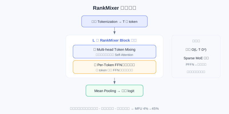
After input features are tokenized, they pass through multiple RankMixer Blocks (each = Token Mixing + Per-Token FFN), and mean pooling finally produces the logit. All core operations are matrix multiplications.
Each RankMixer Block's forward pass:
Overall complexity is . In the Sparse MoE version, the Per-Token FFN can be replaced with expert networks, expanding parameters while keeping inference cost. The design follows three principles: (1) all core operations are matrix multiplications, fully exploiting Tensor Cores; (2) the computation graph stays as simple as possible to reduce kernel launch overhead; (3) the expressiveness required by recommendation tasks is preserved.
7.4.1 The Token Mixing Mechanism
Self-Attention complexity is (from computing the full token-pair similarity matrix ). In recommendation, feature counts can reach hundreds or thousands, making the term a significant bottleneck. RankMixer's core insight: what recommendation tasks need is information mixing between tokens, not similarity-based dynamic weighting (attention). For example, learning high-order interactions like "young users in tier-1 cities prefer tech items" is essentially fusing information from multiple tokens into new representations — it does not necessarily require explicitly computing token-pair similarities.
Token Mixing's core idea: mix along the feature dimension rather than the token dimension. Given input , there are two steps:
Step 1, Multi-head decomposition — each token is decomposed into heads: , where is head of token .
Step 2, Token-wise mixing — within each head, concatenate that head's portion across all tokens: .
The key: change the data layout from "per token" to "per head". The original is vectors of length ; after SplitHead+Concat it becomes vectors of length , with different tokens' features densely packed within each head, creating the conditions for mixing. In practice , so each "head" holds a slice of every token's features. After mixing the token count is unchanged, enabling residual connections.
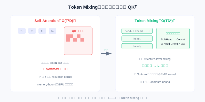
Left: Self-Attention computes the full similarity matrix (); right: Token Mixing rearranges by head and applies a linear transformation along the feature dimension (), with no softmax.
Complexity-wise, Token Mixing costs (mainly memory rearrangement). Compared with self-attention's , this avoids the term when is large (hundreds to thousands in recommendation) — a significant reduction. And Token Mixing has no softmax normalization (which requires an extra reduction kernel), further cutting kernel overhead.
The key question: without explicitly computing token-pair similarities, how are interactions still captured? The answer is stacking multiple layers. A single Token Mixing layer is "feature-level mixing" — the same feature dimension across tokens influences each other (because they are concatenated into one vector). With multiple stacked layers, layer 1's per-token output fuses first-order information from all tokens; layer 2's input is already a mixed result where each token contains other tokens' information, so layer 2's mixing achieves second-order interactions:
Each Token Mixing layer applies a linear transformation along the feature dimension (followed by FFNs), so stacking layers can model -th order polynomial interactions between tokens. In practice is usually 6–12 layers, enough to capture the needed high-order crossings.
From the hardware's perspective, Token Mixing's core is data rearrangement (SplitHead, Concat) that can be implemented with efficient kernels, designed as contiguous memory reads/writes (coalesced memory access) to fully use bandwidth. Compared with attention's softmax (a global normalization), Token Mixing is local and parallel. More importantly, SplitHead, Concat, and the FFN can be fused into a single kernel, reducing kernel launch overhead — the key to the MFU improvement.
Analysis: Token Mixing replaces "token-pair similarity + softmax" with "feature-dimension mixing + multi-layer stacking", dropping to overall, with all operations fusable into matrix-multiply kernels. What is sacrificed is attention's "dynamic similarity routing"; what is gained is GPU utilization — for recommendation, where features are numerous and interaction patterns fairly fixed, this trade is well worth it.
7.4.2 Per-Token FFN
The standard Transformer's FFN uses the same weights for all tokens: . This is reasonable for LLMs (all tokens share one semantic space). But recommendation features live in entirely different semantic spaces: user IDs imply implicit preferences, item categories are coarse-grained classes, click rates follow long-tail distributions, timestamps have periodicity. Forcing the same FFN on them loses parameter efficiency.
RankMixer's core design: each token gets its own FFN parameters. For the -th token:
Each token's is independent, so: (1) each token learns a transformation specific to its semantic space; (2) high-information tokens are automatically allocated more parameter capacity; (3) different semantic spaces no longer interfere.
Per-Token FFN is fundamentally different from MMoE. In MMoE, multiple experts share the same input, and gating dynamically weights a combination of expert outputs: (all experts see the same ). Per-Token FFN gives each token its own input and its own FFN: (each FFN sees a different ). Parameter isolation ensures learning in different feature spaces stays independent, preventing high-frequency features from dominating low-frequency ones.
For parameter efficiency, with tokens, Per-Token FFN has total parameters — times the shared FFN's (). But computational complexity is unchanged: , identical to the shared FFN (which must also compute once per token for tokens). The added parameters are "specialized" — each block serves only one token, giving higher learning efficiency.
Cross-feature-space interaction happens through the Token Mixing layers. Per-Token FFN focuses on deep modeling within each space; Token Mixing ensures information flows between tokens. This "mixing + per-token processing" combination preserves parameter isolation while achieving thorough cross-space interaction through multi-layer stacking.
7.4.3 Sparse MoE Scaling
With Token Mixing and Per-Token FFN in place, how do we scale to billions or even tens of billions of parameters? Directly adding depth/width scales compute linearly, and inference latency grows proportionally — industrially unacceptable. Sparse MoE (Sparse Mixture of Experts) provides the solution: not all parameters participate in every sample's computation; a subset of experts is dynamically selected per sample. The model can have a huge parameter count while per-sample compute stays fixed (activating only a few experts).
The ideal MoE pattern has each expert specialize in some sample pattern. But achieving effective expert specialization in recommendation faces three challenges: (1) the input is high-dimensional sparse features whose combinatorial space is exponential; representations are scattered across the high-dimensional space without clear cluster structure, making stable routing hard for the gating to learn; (2) data is extremely imbalanced — head users account for 50% of samples; if gating routes many head samples to one expert early on, that expert receives more gradients, gating keeps sending it more, and a few experts end up processing most samples (expert overload) while the rest go nearly unused (expert underutilization); (3) even if training is load-balanced, request distributions at inference may differ, making some experts bottlenecks and increasing latency variance.
RankMixer counters with two complementary training strategies. First, ReLU Routing — standard MoE uses Top- + Softmax routing, activating a fixed experts per token. RankMixer's ReLU Routing lets each token activate a variable number of experts:
ReLU outputs can be 0 (not activated) or positive (activated), so high-information tokens may activate more experts. To control sparsity, a regularization is added: , where and controls the average number of activated experts.
Second, Dense-Training / Sparse-Inference (DTSI-MoE) — Per-Token FFN already multiplies parameters by ; adding MoE on top expands expert count further, easily causing expert under-training. DTSI-MoE uses two routers: during training, a dense router activates all or most experts to ensure sufficient training; at inference, a sparse router activates only a few experts to cut compute. Both routers train simultaneously; only is constrained by :
During training, the forward pass uses while is computed alongside and given the sparsity regularization; at inference, only is used. This achieves sufficient training, efficient inference, and consistent strategy.
Load balancing is achieved through the soft constraint of . Expert 's total activation in a batch is , and the regularization can be rewritten as . When some expert's grows too large, the gradient suppresses its activation probability, achieving load balance. Compared with hard constraints (capacity limits), a soft constraint never force-assigns suboptimal experts when one is saturated, preserving routing flexibility.
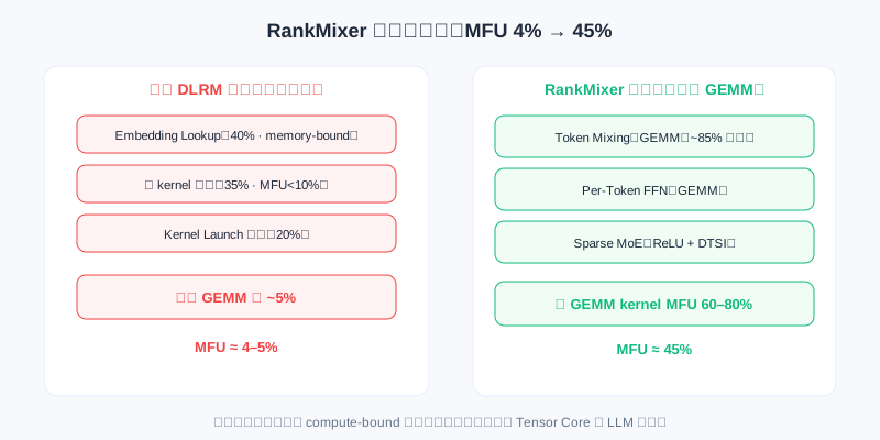
Left: the traditional DLRM's fragmented computation graph (memory-bound embedding lookups, small kernels, launch overhead), with effective GEMM at only 5%; right: RankMixer's core operations are all GEMMs — Token Mixing + PFFN take ~85% of compute, and MFU reaches 45%.
The key to RankMixer's high MFU: all core operations are compute-bound large matrix multiplications. Token Mixing and PFFN take about 85% of compute time, all GEMMs that efficiently use Tensor Cores (a single GEMM kernel reaches 60–80% MFU). By contrast, in the traditional DLRM, embedding lookups (40% of time, memory-bound), small kernels (35% of time, MFU<10%), and launch overhead (20% of time) dominate, with effective GEMM at only 5% — which is exactly why a DLRM's MFU is 4–5% while RankMixer reaches 45%.
💡 Key Insight: RankMixer moves the recommendation model from fragmented design to a unified architectural paradigm. Algorithmically, Token Mixing drops complexity from to , Per-Token FFN captures feature heterogeneity, and Sparse MoE achieves parameter-efficient scaling through ReLU Routing and DTSI-MoE. Systematically, unifying all core operations as matrix multiplications raises MFU from 4–5% to 45%, making the recommendation model a "first-class citizen" on GPU that can directly use Tensor Cores and the mature LLM toolchain, opening a path to sustained scaling. But RankMixer focuses on compute efficiency inside the model; the pipeline still has other fragmentation — sequence modeling separate from feature interaction, retrieval separate from ranking, multi-task fragmentation. The next section, OneTrans, breaks through these remaining walls.
⚠️ Common Mistakes in 7.4
| # | Mistake | Example | Why It's Wrong | Fix |
|---|---|---|---|---|
| 1 | Assuming low MFU just means few parameters | "Add GPUs and utilization is solved" | It is architectural fragmentation + memory-bound access, not a shortage of compute | Use hardware-aware unification into GEMMs |
| 2 | Assuming Token Mixing loses interactions | "Without token-pair similarity there are no crossings" | Multi-layer stacking achieves -th order polynomial interactions | Look at the stacking |
| 3 | Treating Per-Token FFN as MMoE | "One expert per token is just MoE" | MMoE shares the input and weights combinations; PFFN gives each token independent input/parameters | Distinguish parameter isolation from routed weighting |
| 4 | Using Top-k Softmax routing | "MoE should always activate a fixed k" | Sparse recommendation features make stable routing hard, and imbalance causes overload | Use ReLU Routing for dynamic activation |
| 5 | Ignoring the necessity of DTSI-MoE | "Just train sparse directly" | PFFN already multiplies parameters by T; pure sparse training under-trains experts | Two routers: dense training, sparse inference |
Chapter Summary
📌 Key Takeaways
| Concept | Key Points | Why It Matters |
|---|---|---|
| The MFU bottleneck | DLRM only 4–5%, LLM 40–60% | The hardware root cause of recommendation's scaling trouble |
| Token Mixing | Feature-dimension mixing replaces , complexity | Removes the term + fusable kernels |
| Per-Token FFN | Independent FFN parameters per token, unchanged complexity | Captures feature heterogeneity, parameter isolation |
| Sparse MoE | ReLU Routing + DTSI-MoE | Parameter-efficient scaling to the billion level |
| Unify as GEMM | All core operations are matrix multiplications | MFU up to 45%, a first-class GPU citizen |
❓ FAQ
Q1: Without computing similarities, can Token Mixing really replace Self-Attention?
A: Yes. High-order crossings in recommendation are essentially "fusing multiple tokens' information into new representations"; a single layer mixes along the feature dimension, and stacking layers achieves -th order polynomial interactions. The cost is losing dynamic similarity routing, but with many features and relatively fixed patterns in recommendation, the gained GPU utilization is the better deal.
Q2: Per-Token FFN multiplies parameters by T — why don't FLOPs change?
A: A shared FFN also computes once per token for T tokens (one FFN per token), so FLOPs were already ; Per-Token merely swaps the shared weights for T independent sets, still computing once per token — same FLOPs. What grows is "specialized" parameters with higher learning efficiency.
Q3: Why does recommendation MoE use ReLU Routing instead of Top-k?
A: Recommendation inputs are high-dimensional, sparse, and unevenly distributed; Top-k's fixed activation count easily overloads a few experts while the rest go underutilized. ReLU lets each token activate a variable number of experts based on information content, and with the regularization it achieves soft load balancing — better suited to recommendation data.
🔗 Connections to Later Chapters
- 7.3 (MTGR) — also handles heterogeneous features, but with GLN + Dynamic Masking; compare with RankMixer's Per-Token FFN (separate parameters) approach.
- 7.5 (OneTrans) — further breaks the fragmentation of "sequence modeling separate from feature interaction", extending RankMixer's hardware thinking to a unified architecture.
- 3.2 (Feature Crossing) — the high-order crossings of DCN/xDeepFM are re-implemented in RankMixer via multi-layer Token Mixing, and in a more GPU-friendly way.
Practice Problems
Work through all problems in order — they get progressively harder. Each has a complete solution you can reveal after trying it yourself.
Problem 7.4.1 — The Root Cause of Low MFU 🟢 Easy
A traditional DLRM's MFU is about 4–5%, an LLM's about 40–60%. Name the three architecture-level causes of the DLRM's low MFU.
💡 Solution (click to reveal)
Approach: Map to the three fundamental problems in the text.
- Core operations are memory-bound (embedding lookup, feature crossing — memory traffic >> compute);
- The computation graph is highly fragmented (many independent modules chained; kernel launch + global memory transfer overhead);
- Tensor Cores are underutilized (small vectors/irregular access, not GEMM).
Key points:
- It is not a lack of compute; the compute is not "worth it".
- RankMixer's unification into GEMM pulls MFU to 45%.
Problem 7.4.2 — Token Mixing Complexity 🟢 Easy
Self-Attention complexity is and Token Mixing about (rearrangement). With , by about how many times do the orders of magnitude differ?
💡 Solution (click to reveal)
Approach: Substitute and estimate (ignore constants).
- Self-Attention: .
- Token Mixing: .
- The ratio is x (i.e., times).
Key points:
- Token Mixing removes the term and scales linearly with token count.
- In recommendation, T is hundreds to thousands — the gain is significant.
Problem 7.4.3 — Per-Token FFN vs MMoE 🟡 Medium
Why are Per-Token FFN and MMoE "fundamentally different"? Summarize each one's parameter organization in a sentence.
💡 Solution (click to reveal)
Approach: Distinguish "parameter isolation" from "routed weighting".
- MMoE: multiple experts share the same input , and gating dynamically weights the output combination — all experts see the same input.
- Per-Token FFN: each token has its own input and its own FFN — parameter isolation, preventing high-frequency features from dominating low-frequency ones.
Key points:
- One is "same input, weighted expert selection"; the other is "different inputs, each with its own FFN".
- Both aim to handle heterogeneous features; the mechanisms differ.
Problem 7.4.4 — DTSI-MoE Design 🔴 Hard
Explain why DTSI-MoE needs two routers ( and ), and what would happen if you trained with only .
💡 Solution (click to reveal)
Approach: Start from the tension between "sufficient training vs efficient inference".
Per-Token FFN already multiplies parameters by T, and MoE expands the expert count further; if training also activates sparsely, many experts never receive enough gradients → expert under-training. DTSI-MoE uses during training to activate most experts (sufficient training), while only is constrained by the sparsity regularization and used at inference. Training with only would under-train the experts, and the deployed model would perform poorly.
Key points:
- Dense training preserves quality; sparse inference preserves efficiency.
- The two routers train simultaneously with a consistent strategy.
🏆 Challenge: Hardware-Aware Restructuring
You must restructure a fragmented DLRM (embedding lookup + hand-crafted crossing + DIN + MLP) into a GPU-friendly architecture. Within 150 words, state which three RankMixer components you would substitute for the existing modules, and the expected MFU change plus its precondition.
💡 Hint
Replace Self-Attention/hand-crafted crossing with Token Mixing (removes , fusable kernels), replace the shared FFN with Per-Token FFN (captures feature heterogeneity), and scale parameters with Sparse MoE. The precondition is first tokenizing all features and unifying the computation graph as matrix multiplications; expect MFU to rise from ~5% to ~45%. This corresponds exactly to RankMixer's hardware-aware restructuring approach.