Word2Vec Deep Dive
📝 Why this is a separate appendix: Section 2.2.1 of 2.2 Vector Retrieval (I2I) covers only the Skip-Gram intuition and its transfer to recommendation. This appendix fills in what was left out — the CBOW architecture, the structural details of the two center/context embedding tables, the precise mathematical form of negative sampling, and the arithmetic (analogy) properties of word vectors — so that you thoroughly understand the underlying engine before using Item2Vec / EGES / Airbnb.
The goal of Word2Vec is plain: from large amounts of unlabeled text, learn a low-dimensional dense vector for every word such that:
- semantically similar words end up close to each other in the vector space;
- relations between words are reflected through vector arithmetic.
These representations can be fed directly into downstream tasks such as text classification, machine translation, and information retrieval — and in recommendation, the method was transferred "structurally isomorphically" into Item2Vec.
1. Motivation: From One-Hot to Dense Vectors
The earliest and most direct approach encodes words with one-hot encoding: with a vocabulary size of , the -th word is a -dimensional vector with a 1 in position and 0s elsewhere. It is intuitive but has three fatal flaws:
| Flaw | Explanation |
|---|---|
| Curse of dimensionality | often reaches the millions; the vectors are huge and sparse |
| No semantics | The one-hot inner product of any two different words is 0, so "cat" and "dog" are treated as unrelated |
| No syntax | Relations such as singular/plural and tense are lost entirely |
What we need is a representation that is both low-dimensional and able to carry semantic/syntactic information — exactly the problem Word2Vec solves.
2. The Distributional Hypothesis and the Context Window
The theoretical foundation of Word2Vec is the linguistic distributional hypothesis (Firth, 1957):
"You shall know a word by the company it keeps." The meaning of a word is determined by the words that appear around it.
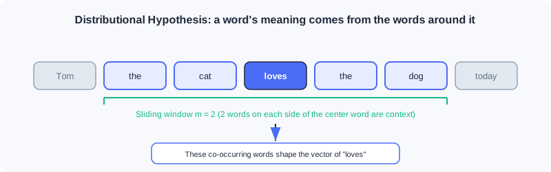
The model walks through every word in the corpus and adjusts the word vectors so that the "predicted context" matches the "actual context in the corpus" as closely as possible. Concretely, if the center word sits at position , its context is the words within the window : .
3. Two Architectures: Skip-gram and CBOW
Word2Vec comprises two mirror-symmetric models. In 2.2.1 we used only Skip-Gram; here we add CBOW as well.
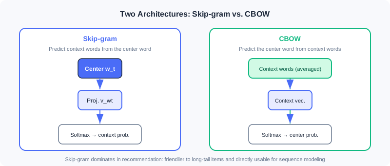
3.1 Skip-gram: Predict the Context from the Center Word
Given a center word, the model predicts the probability of its context words appearing. For a context word inside the window, the conditional probability is
where is the vector representation of word and is the vocabulary size. Walking through the whole corpus, the likelihood is
3.2 CBOW: Predict the Center Word from the Context
CBOW (Continuous Bag of Words) goes the other way: it averages the context words and predicts the center word.
💡 Which one should you use? Recommendation scenarios almost always use Skip-gram, for two reasons: ① it is friendlier to low-frequency/long-tail words (every context pair provides an independent supervision signal); ② it naturally fits variable-length, sparse inputs like user behavior sequences and can be used for sequence modeling directly. CBOW averages the context and would wipe out sequence-order information in recommendation.
4. Model Structure and the Two Embedding Tables
The conditional probability formulas above hide a detail that is very easy to get wrong: the center-word vector and the context-word vector do not live in the same vector space.
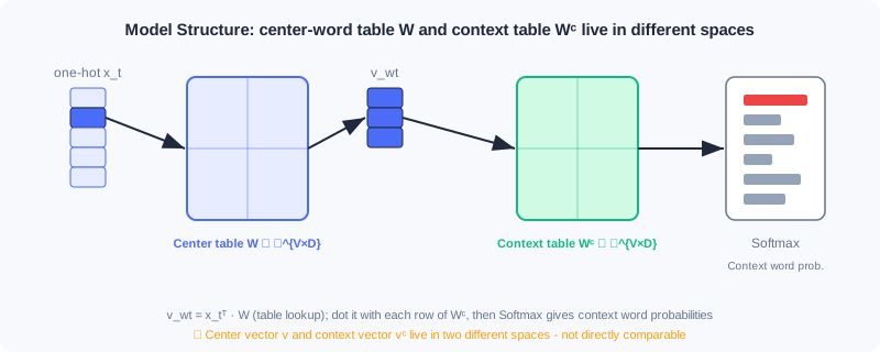
Taking Skip-gram as an example, let the vector dimension be ; there are two embedding tables:
- the center-word table
- the context-word table
The forward computation proceeds as follows:
- Input the one-hot representation of the center word;
- Look up the center-word vector ;
- Multiply with row of the context-word table to get the input to the Softmax;
- Apply the Softmax to output context-word probabilities.
⚠️ Common Mistakes in Word2Vec Treating (from ) and (from ) as vectors in the same space and directly computing distances. They come from two different tables; only the "final word vectors" obtained by adding/averaging the two tables after training are valid for similarity computation.
5. Negative Sampling: Making Softmax Computable
Computing the Softmax denominator from Sections 3/4 directly requires iterating over the entire vocabulary (millions of entries), which is unaffordable. Word2Vec uses negative sampling to decompose the multi-class problem into many binary-class problems.
Taking Skip-gram as an example, the original objective is replaced with:
where is the sigmoid, is the number of negative samples, and is the negative sampling distribution. The original paper takes
💡 Intuition: The first term pushes the similarity of "true context word pairs" higher (lifting positive samples); the second pushes the similarity of "randomly sampled negative word pairs" lower (suppressing negatives). By the monotonicity of the sigmoid, this is consistent with maximizing the original likelihood , yet it avoids summing over the entire vocabulary — the complexity drops from to .
⚠️ Common Mistakes in Word2Vec Assuming that negative sampling is just a "speed trick" with no semantic effect. In fact, the 3/4 power in the negative sampling distribution deliberately lifts the probability of low-frequency words being drawn as negatives, so that the model learns discriminative vectors for rare words too — which is especially critical for long-tail items in recommendation.
6. Vector Arithmetic: The Analogy Property
The most fascinating discovery about Word2Vec is that in the trained vector space, semantic relations can be expressed through vector addition and subtraction. The classic example:
This means that analogies like "king − man + woman ≈ queen" are encoded into the geometric structure. In recommendation, the analogous property reads as "the difference between item A and item B roughly equals the difference between item C and some item D" — exactly the theoretical grounding that later lets semantic IDs and vector retrieval perform "computable analogies".
7. From Word2Vec to Recommendation: The Item2Vec Bridge
Transferring Word2Vec to recommendation takes just one structural isomorphic substitution (details in 2.2.1):
| Text world | Recommendation world |
|---|---|
| Word | Item |
| Sentence | User interaction sequence |
| Word co-occurrence | Items interacted with by the same user |
After the substitution:
- Skip-gram + negative sampling → becomes the training prototype of Item2Vec directly;
- the learned item vectors → enable I2I retrieval through nearest-neighbor search;
- the two-table structure and the negative sampling distribution from Sections 4–5 intact underpin industrial variants such as EGES and Airbnb.
💡 One-sentence takeaway: The Word2Vec engine (Skip-gram + two embedding tables + negative sampling) is the methodological cornerstone of I2I vector retrieval; every improvement in the recommendation domain only plays with "how to construct sequences" and "how to define positive and negative samples".
Chapter Summary
- Word2Vec uses the distributional hypothesis to turn "co-occurrence" into "dense semantic vectors", fixing the three flaws of one-hot: high dimensionality, sparsity, and no semantics.
- Two architectures: Skip-gram (center → context) and CBOW (context → center); recommendation almost always uses Skip-gram.
- Structurally there are two embedding tables, (center) and (context), belonging to different spaces; the final vectors must be merged before use.
- Negative sampling approximates the full-vocabulary Softmax with binary classifications and lifts low-frequency words via — the key to industrial feasibility.
- Word vectors support analogical arithmetic, providing the theoretical underpinning for semantic IDs and vector retrieval.
- Through the isomorphic substitution "word → item, sentence → behavior sequence", Word2Vec becomes the engine of Item2Vec and the subsequent I2I methods directly.
🔗 Connections to Later Chapters
- Prerequisite: Section 2.2.1 of 2.2 Vector Retrieval (I2I) cites this appendix briefly as the "theoretical basis of sequence modeling"; after reading the appendix, revisiting that section will make it clearer why Item2Vec / EGES / Airbnb are designed the way they are.
- What follows: 2.3 Two-Tower Models (U2I) retrieves with dense vectors from a "user tower + item tower", carrying forward the "dense item vectors" idea here; 6.4 Codebook Quantization and Semantic IDs inverts "discrete words → continuous vectors" into "continuous vectors → discrete semantic IDs" — worth reading side by side.
Practice Problems
Problem A.1 — The two-table misconception 🟢 Easy
Someone says: "In Word2Vec, the vectors of the center word and the context word live in the same -dimensional space, so you can just compute the cosine similarity directly." What is wrong with this claim?
Approach: Revisit Section 4 — comes from , while comes from .
Answer: The mistake is assuming the two share one space. In reality, the center-word table and the context-word table are two independent parameter tables, and their vectors belong to different spaces; comparing distances directly is invalid. After training, the two tables are usually added/averaged into the final word vectors, and only those are valid for similarity computation.
Problem A.2 — Negative-sampling scaling 🟡 Medium
The negative sampling distribution uses rather than raw word frequency. If one word appears 16 times and another appears 81 times, compute their relative weight ratio after the power (i.e., ), and explain the effect of this design on low-frequency words.
Approach: ; .
Answer: The relative weight ratio is . Note that the frequency ratio is ; after the power the gap gets compressed (5.06 → 3.375), which effectively lifts the probability of low-frequency words being drawn as negative samples — so the model learns discriminative vectors for rare words too, easing the long-tail problem.
Problem A.3 — Isomorphic transfer 🔴 Hard
When transferring Word2Vec to recommendation as Item2Vec, why is the mapping "user interaction sequence = sentence" a structural isomorphism rather than a loose analogy? Explain from the perspective of the training objective (Skip-gram + negative sampling), and point out one key simplification of Item2Vec relative to the original Word2Vec mentioned in 2.2.1.
Approach: Isomorphism means a one-to-one correspondence across "input units + co-occurrence structure + training objective"; the key simplification is that Item2Vec treats user history as an unordered set rather than a sequence.
Answer: The isomorphism shows up as: word → item, sentence → user behavior sequence, word co-occurrence → same-user interactions, while the Skip-gram + negative-sampling objective is unchanged in form — only the text corpus is swapped for a behavior-sequence corpus. Key simplification: as noted in the book, Item2Vec by default treats each user's interaction history as an unordered set (ignoring temporal order), whereas the original Word2Vec strictly depends on ordered context within the sliding window — this is the most essential difference from the text version.