Diffusion Model Basics for Recommendation

📝 Before You Continue: Read the two paradigms in 1.1 and the generative paradigm evolution in 5.3 first. This chapter is the "technical groundwork" for deploying diffusion in recommendation; the concrete methods in 10.2/10.3 all build on it.

In 5.3 we discussed, at the architecture level, how diffusion models and Transformers complement each other. This section systematically reviews the core technical principles of diffusion models, with emphasis on the special considerations and design choices when applying them to recommendation. The theoretical foundation comes mainly from DDPM, while DiffRec is the representative work for recommendation applications.

The core idea of diffusion models can be summarized as two inverse Markov processes: forward diffusion gradually adds noise to data, and reverse denoising learns to recover the original data from noise. After reading this section, you will understand this mechanism and why it can serve as a "generative tool" for recommender systems.

After reading this section, you will be able to:

• Write the single-step transition of forward diffusion and the direct sampling formula for any t (reparameterization)
• Distinguish data-space diffusion from latent-space diffusion, and explain why recommendation prefers the latter
• Describe the ELBO training objective and the two parameterizations: ε-prediction and x₀-prediction
• Explain noise scale control in recommendation, inference starting-point selection, conditional generation, and the two guidance strategies
• Complete 4 tiered practice problems, and try the interactive "forward/reverse" demo at the end

10.1.0 Two Operating Spaces of Diffusion Models

By operating space, diffusion models fall into two main families:

Data-space diffusion (pixel-space diffusion) — diffusion and denoising happen directly in the raw data space (image pixels; interaction vectors in recommendation). The representative work is DDPM. It is theoretically more direct, but iterating in a high-dimensional raw space is computationally expensive, and it is especially inefficient for high-resolution data or long sequences.

Latent diffusion models (LDM) — an encoder (VAE / autoencoder) first compresses the raw data into a low-dimensional latent representation space; diffusion and denoising happen there, followed by decoding back to the original space. The representative work is Stable Diffusion. Pipeline: encode $\mathbf{z}=\mathcal{E}(\mathbf{x})$ → diffuse on $\mathbf{z}$ → decode $\hat{\mathbf{x}}=\mathcal{D}({\mathbf{z}}_0)$. If the dimension drops from $d$ to $d^{\prime }$ ($\ll d$), the computation can shrink by a factor of $(d/d^{\prime }{)}^2$.

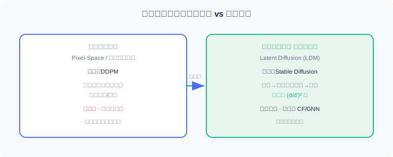
💡 Key Insight: In recommendation, latent diffusion is far more common, for three reasons: ① efficiency — recommendation deals with large-scale behavior sequences and item features, so operating in the raw space is unacceptable; ② semantics — the latent space offers a more compact, semantic representation that fits user interest / item attribute modeling; ③ flexibility — it integrates easily with existing architectures such as CF and GNN. Hence the methods in this part mostly diffuse in item embedding or user feature spaces rather than operating directly on the sparse interaction matrix.

10.1.1 Forward Noising and Reverse Denoising

The Forward Diffusion Process

Given a data sample ${\mathbf{x}}_0\sim q({\mathbf{x}}_0)$, the forward process adds Gaussian noise over $T$ steps, building latent variables ${\mathbf{x}}_{1:T}$. Each step transitions as:

$$q({\mathbf{x}}_t|{\mathbf{x}}_{t-1})=\mathcal{N}({\mathbf{x}}_t;\sqrt{1-{\beta }_t}{\mathbf{x}}_{t-1},{\beta }_t\mathbf{I})$$

where ${\beta }_t\in (0,1)$ controls the noise strength at step $t$. As $T\to \infty$, ${\mathbf{x}}_T$ approaches a standard Gaussian. Using the reparameterization trick and the additivity of Gaussians, we can sample the noised data at any $t$ directly from ${\mathbf{x}}_0$:

$$q({\mathbf{x}}_t|{\mathbf{x}}_0)=\mathcal{N}({\mathbf{x}}_t;\sqrt{{\bar{\alpha }}_t}{\mathbf{x}}_0,(1-{\bar{\alpha }}_t)\mathbf{I})$$

Equivalently:

$${\mathbf{x}}_t=\sqrt{{\bar{\alpha }}_t}{\mathbf{x}}_0+\sqrt{1-{\bar{\alpha }}_t}\mathbf{ϵ},\mathbf{ϵ}\sim \mathcal{N}(0,\mathbf{I})$$

where ${\alpha }_t=1-{\beta }_t$ and ${\bar{\alpha }}_t={\prod }_{i=1}^t{\alpha }_i$. This allows efficient sampling of any timestep during training, without executing the forward process step by step.

The Reverse Denoising Process

The reverse process starts from ${\mathbf{x}}_T$ and gradually recovers the original data through a learned denoising network. Each denoising step transitions as:

$$p_{\theta }({\mathbf{x}}_{t-1}|{\mathbf{x}}_t)=\mathcal{N}({\mathbf{x}}_{t-1};{\mathbf{\mu }}_{\theta }({\mathbf{x}}_t,t),{\mathbf{\Sigma }}_{\theta }({\mathbf{x}}_t,t))$$

The mean ${\mathbf{\mu }}_{\theta }$ and covariance ${\mathbf{\Sigma }}_{\theta }$ are parameterized by a neural network; in practice the covariance is often fixed as ${\sigma }^2(t)\mathbf{I}$, and the mean is the focus of learning.

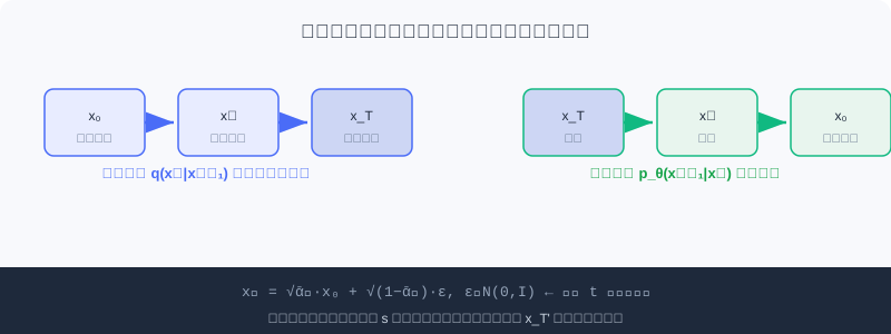
The interactive demo below lets you see how a "user interaction vector" is gradually noised into static and then recovered by denoising:

Click "Next step" or "Autoplay" and watch the signal cells — a clear interaction pattern in the forward pass — get progressively drowned in noise, then recovered by reverse denoising. This is the full process of a diffusion model "sculpting" the target data.

10.1.2 Training Objective and Two Parameterizations

From ELBO to the Simplified Loss

Diffusion models are trained by maximizing the evidence lower bound (ELBO) of the log-likelihood of ${\mathbf{x}}_0$:

$$\log p({\mathbf{x}}_0)\ge \underset{\text{reconstruction term}}{\underbrace{{\mathbb{E}}_{q({\mathbf{x}}_1|{\mathbf{x}}_0)}[\log p_{\theta }({\mathbf{x}}_0|{\mathbf{x}}_1)]}}-\sum _{t=2}^T\underset{\text{denoising matching term}}{\underbrace{\mathbb{E}[D_{\text{KL}}(q({\mathbf{x}}_{t-1}|{\mathbf{x}}_t,{\mathbf{x}}_0)\Vert p_{\theta }({\mathbf{x}}_{t-1}|{\mathbf{x}}_t))]}}$$

The reconstruction term measures the ability to recover ${\mathbf{x}}_0$ from ${\mathbf{x}}_1$; the denoising matching term forces the learned reverse transition $p_{\theta }$ to align with the true posterior $q({\mathbf{x}}_{t-1}|{\mathbf{x}}_t,{\mathbf{x}}_0)$. At inference time we do not know ${\mathbf{x}}_0$, so we must train the network $p_{\theta }$ to approximate this ideal process.

Two Parameterizations

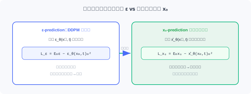
The denoising network can adopt two parameterizations:

1. Predicting the noise $\mathbf{ϵ}$ (the DDPM standard):

$${\mathcal{L}}_{ϵ}={\mathbb{E}}_{t,{\mathbf{x}}_0,\mathbf{ϵ}}[\Vert \mathbf{ϵ}-{\mathbf{ϵ}}_{\theta }({\mathbf{x}}_t,t){\Vert }^2]$$

2. Predicting the original data ${\mathbf{x}}_0$:

$${\mathcal{L}}_{x_0}={\mathbb{E}}_{t,{\mathbf{x}}_0,\mathbf{ϵ}}[\Vert {\mathbf{x}}_0-{\hat{\mathbf{x}}}_{\theta }({\mathbf{x}}_t,t){\Vert }^2]$$

The two are mathematically equivalent (${\mathbf{x}}_t=\sqrt{{\bar{\alpha }}_t}{\mathbf{x}}_0+\sqrt{1-{\bar{\alpha }}_t}\mathbf{ϵ}$), but recommendation often uses x₀-prediction. The reason: the goal in recommendation is to recover the original interactions ${\mathbf{x}}_0$ from the noised interaction vector and directly use ${\hat{\mathbf{x}}}_0$ as the interaction prediction score for ranking; moreover, the random noise $\mathbf{ϵ}$ has high variance, and forcing the network to estimate such an unstable target makes training harder.

The Sampling Process

After training: ① sample ${\mathbf{x}}_T\sim \mathcal{N}(0,I)$; ② iterate denoising for $t=T,\dots ,1$:

$${\mathbf{x}}_{t-1}=\frac{1}{\sqrt{1-{\beta }_t}}\left({\mathbf{x}}_t-\frac{{\beta }_t}{\sqrt{1-{\bar{\alpha }}_t}}{\mathbf{ϵ}}_{\theta }({\mathbf{x}}_t,t)\right)+{\sigma }_t\mathbf{z}$$

③ obtain the generated sample ${\mathbf{x}}_0$.

🧠 Mental Model: The Sculptor and the Block of Stone

Forward diffusion is like gradually hammering an intact marble block into a pile of rubble (noising); reverse denoising is like a sculptor who, guided by an "afterimage," chisel by chisel carves the rubble back into a human figure (denoising). x₀-prediction means the sculptor always imagines directly "what the final figure looks like," which is easier than staring at "the pile of rubble just knocked off" — this is exactly why recommendation prefers it.

10.1.3 Special Designs for Recommendation

Unlike image generation, diffusion in recommendation involves two special designs:

Noise scale control — standard DDPM diffuses data to a pure Gaussian (${\bar{\alpha }}_T\to 0$), but in recommendation completely losing historical preference makes generation harder. So a noise scale parameter $s$ limits the maximum strength, keeping part of the original signal even at $t=T$:

$$1-{\bar{\alpha }}_t=s\cdot \left[{\alpha }_{\min }+\frac{t-1}{T-1}({\alpha }_{\max }-{\alpha }_{\min })\right]$$

Here $s\in (0,1)$ controls the upper bound of the overall noise strength, and ${\alpha }_{\min },{\alpha }_{\max }$ delimit the interval over which the noise ratio grows linearly with $t$ (this design comes from DiffRec and has been widely adopted by subsequent diffusion recommender works).

Inference starting-point selection — inference can start reverse denoising from a partially noised state ${\mathbf{x}}_{T^{\prime }}$ ($T^{\prime }<T$), which both leverages denoising to fix noise in the raw interactions and preserves enough personalization information.

Conditional Generation and Controllability

Recommendation wants generation controlled by user history / context. Conditional information can be injected into the denoising network: direct concatenation, additive fusion, or cross-attention in a Transformer. The conditional loss:

$${\mathcal{L}}_{\text{cond}}={\mathbb{E}}_{t,{\mathbf{x}}_0,\mathbf{ϵ},\mathbf{c}}[\Vert \mathbf{ϵ}-{\mathbf{ϵ}}_{\theta }({\mathbf{x}}_t,t,\mathbf{c}){\Vert }^2]$$

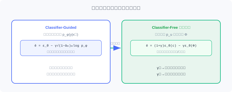
At inference, two main strategies steer the generation direction:

1. Classifier-guided — use gradients of a pretrained classifier $p_{\varphi }(y|{\mathbf{x}}_t)$ to push toward the target class:

$$\widehat{\mathbf{ϵ}}={\mathbf{ϵ}}_{\theta }({\mathbf{x}}_t,t)-\gamma \cdot \sqrt{1-{\bar{\alpha }}_t}{\nabla }_{{\mathbf{x}}_t}\log p_{\varphi }(y|{\mathbf{x}}_t)$$

In recommendation, a sequential recommendation model can serve as the "classifier," guiding generation toward interaction sequences consistent with the history.

2. Classifier-free guidance — during training, replace the condition $\mathbf{c}$ with an empty placeholder $\Phi$ with probability $p_u$; at inference:

$$\widehat{\mathbf{ϵ}}=(1+\gamma )\cdot {\mathbf{ϵ}}_{\theta }({\mathbf{x}}_t,t,\mathbf{c})-\gamma \cdot {\mathbf{ϵ}}_{\theta }({\mathbf{x}}_t,t,\Phi )$$

Large $\gamma$ → more personalized but potentially lower quality; small $\gamma$ → more diverse but less personalized. More commonly used in recommendation.

Example conditional design (sequential recommendation): condition on the user's historical interaction sequence, encode it with a Transformer encoder into ${\mathbf{c}}_{n-1}=\text{T-enc}({\mathbf{e}}_{1:n-1})$, and guide diffusion to generate the target item embedding — combining sequence modeling (Transformer) with generative modeling (diffusion). DreamRec adopts exactly this architecture.

Analysis: In recommendation, diffusion does not primarily aim to end-to-end replace discriminative models; instead, its generative capability + random sampling provides tools for two concrete problems: data sparsity and recommendation diversity. This is the through-line for understanding 10.2/10.3.

⚠️ Common Mistakes in 10.1

Chapter Summary

📌 Key Takeaways

❓ FAQ

Q1: Why does recommendation prefer latent diffusion over data-space diffusion?

A: Interaction vectors in recommendation are high-dimensional and sparse; iterative denoising in the raw space is computationally unacceptable. The latent space is more compact and semantic, integrates easily with CF/GNN, and meets industrial real-time requirements.

Q2: Why does recommendation often use x₀-prediction?

A: The goal of recommendation is to recover the user's original interactions and rank on ${\hat{x}}_0$; x₀-pred is more stable and better matched to the task than estimating the high-variance noise ε.

Q3: How should the γ of classifier-free guidance be tuned?

A: Large γ → better adherence to the condition (strong personalization) but potentially lower generation quality / diversity; small γ → more diverse but less personalized. Balance "relevance vs diversity" according to business needs.

🔗 Connections to Later Chapters

• 1.1 / 5.3 (paradigms and generative models) Diffusion is the "continuous-space denoising" branch of the generative family, complementary to autoregressive generation.
• 10.2 (data augmentation) DiffuASR / Diff-MSR apply this section's foundations to generating pseudo-interactions.
• 10.3 (applications) AsymDiffRec / DMSG apply denoising capability to feature completion and diversity.

Practice Problems

Work through all problems in order — they get progressively harder. Each has a complete solution you can reveal after trying it yourself.

Problem 10.1.1 — Direct Sampling Formula 🟢 Easy

Given ${\mathbf{x}}_0$, at step $t$ we have ${\bar{\alpha }}_t=0.6$ and sampled noise $\mathbf{ϵ}\sim \mathcal{N}(0,I)$. Write the expression for ${\mathbf{x}}_t$ and state the relative magnitudes of the signal and noise terms.

Problem 10.1.2 — Choosing the Space 🟢 Easy

For each scenario below, should you prefer data-space or latent-space diffusion? Briefly justify.

• (a) Denoising 1024×1024 high-resolution images
• (b) Recommendation augmentation on a million-dimensional sparse user-item interaction matrix

Problem 10.1.3 — Comparing Parameterizations 🟡 Medium

A diffusion recommender trained with ε-prediction shows large fluctuations in prediction scores and unstable ranking performance. Explain the likely cause, and why switching to x₀-prediction is more appropriate (cite variance and the task objective).

Problem 10.1.4 — Designing Conditional Guidance 🔴 Hard

You need to design a conditional diffusion for sequential recommendation: use a Transformer to encode the user history as the condition $\mathbf{c}$, guiding diffusion to generate the next item embedding. Write down: ① how the condition is injected into the denoising network (at least two ways); ② the training and inference formulas of classifier-free guidance; ③ whether γ should be larger or smaller if you want "more personalization while accepting slightly lower diversity."

🏆 Challenge: Arguing About Recommendation Latency

Diffusion inference requires multi-step iterative denoising, while industrial recommendation often demands sub-second (hundred-millisecond) latency. In 200 words or fewer, argue: for the two use cases "data augmentation (offline)" and "online ranking," is the latency cost of diffusion acceptable in each? Point out one accelerated sampling technique that 10.3 will use.